Help with SUMIFS & INDEX/MATCH Formulas

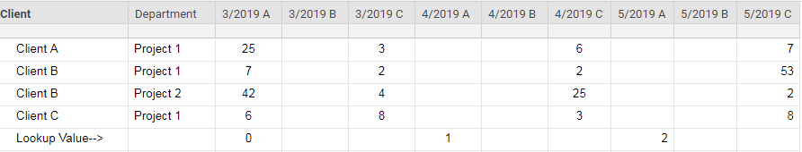
I need to first find the column number where the number 1 resides on the "Lookup Value -->" row.
Next, I need to shift two columns to the right, which would be "4/2019 C" and sum the values for Client B,
I have tried various combinations of SUMIFS, INDEX(MATCH()), etc.,but with my last attempt, I received #INVALID VALUE with the following formula:
=SUMIFS(INDEX(Client1:[5/2019 C]4, MATCH(1, Client5:[5/2019 C]5, 0) + 2), Client1:Client4, "Client B")
Please help! Thank you.
Comments
-
Can you provide a screenshot with some dummy data in it that shows what you want this to look like?
-
Hi Paul,
Please let me know if you cannot see the posted dummy data that I posted with my inquiry.
I have three columns for each month; the first is for user input, the second is for projected hours, and the last one is for actual hours.
With the example posted, Client B during the month of April (4/2019 C) has a sum of 27 (2+25).
I have already written a formula to compare each month to the current month. On the "Lookup Value -->" row, 0 = current month, 1 = next month, 2 = 2 months from current month. This means, on 4/1/2019, Column "4/2019 A" will change from 1 to 0.
Due to the "Lookup Value -->" row changing every month, the column to sum will continue to change. The formula I am trying to write is to find the "Lookup Value -->" with the value of 1. Once it sees this value, I want it to look 2 columns to the right and sum up the data which meets the criteria in my posted formula (below).
Rationale behind my posted formula:
=SUMIFS(INDEX(Client1:[5/2019 C]4, MATCH(1, Client5:[5/2019 C]5, 0) + 2), Client1:Client4, "Client B")
Indexing all of the data, find "1" on the "Lookup Value -->" row. Then look over 2 columns. Then sum the data which equates to "Client B".
The formula I am currently using to acquire this result is absolutely HUGE, hence I was hoping to simplify the formula. This Smartsheet keeps crashing due to multiple uses of my large formula.
Thanks for inquiring! - Dan
-
Ok. So in summary... You want to find the 1, move two columns to the right, and then sum everything in that column?
Sorry if it seems I am asking for a lot of clarification. I just want to make sure we are getting this right. Don't want to waste a lot of time coming up with a "solution" that in all reality doesn't accomplish what you need.
-
Hi Paul.
No, we are not looking to sum the entire column. In this example, we are only looking to sum the values of Client B. We will then use the same formula to look for Client A & Client C in different cells.
Thanks again. - Dan
-
Ok. I've got it now. I have a few ideas but will need a little time for testing and working the details out. I'll get back to you unless someone else is able to come up with a solution before I can.
-
Ok. So I am going to suggest a helper column. For this example I'll name it "Current". I am also going to assume the final column is [12/2019 C]. I am also going to move the row containing the Lookup Value to row 1 since I can't see your current row numbers. You can adjust this to match what you need.
In the Current Column, enter the following:
=INDEX([3/2019 A]@row:[12/2019 C]@row, 1, MATCH(1, [3/2019 A]$1:[12/2019 C]$1, 0) + 2)
This will pull the number from the corresponding row that is two columns to the right of the column containing 1. Note: It is important to keep the row reference in the MATCH function locked using the $. This way you can dragfill the rest of the way down the Current Column.
From there you can use a basic
=SUMIFS(Current:Current, Client:Client, "Client B")
to sum ever cell in the Current column that has "Client B" in the Client column on the same row.
-
Paul,
This is perfect! Thank you so much for your assistance!
Thanks,
Dan
-
Happy to help!

Out of curiosity... What are you using to move the 0, 1, and 2 across the columns?
-
Since I am not using the Date format columns for these, I simply put 3 in [3/2019 A] for March and 2019 in [3/2019 C].
=IF(YEAR(TODAY()) < [3/2019 C]@row, 12 - (12 + [3/2019 A]@row - MONTH(TODAY())), IF(YEAR(TODAY()) = [3/2019 C]@row, (12 + [3/2019 A]@row - MONTH(TODAY())) - 12, [3/2019 A]@row - (12 + MONTH(TODAY()))))
I know it still needs some work. I am concerned with the yearly rollover. Any suggestions?

Help Article Resources
Categories
- All Categories
- 14 Welcome to the Community
- 10.7K Get Help
- 63 Global Discussions
- 68 Industry Talk
- 385 Announcements
- 3.5K Ideas & Feature Requests
- 55 Brandfolder
- 125 Just for fun
- 50 Community Job Board
- 464 Show & Tell
- 40 Member Spotlight
- 44 Power Your Process
- 28 Sponsor X
- 234 Events
- 7.3K Forum Archives
Check out the Formula Handbook template!