Formulas - Can you exclude rows from average calculations?

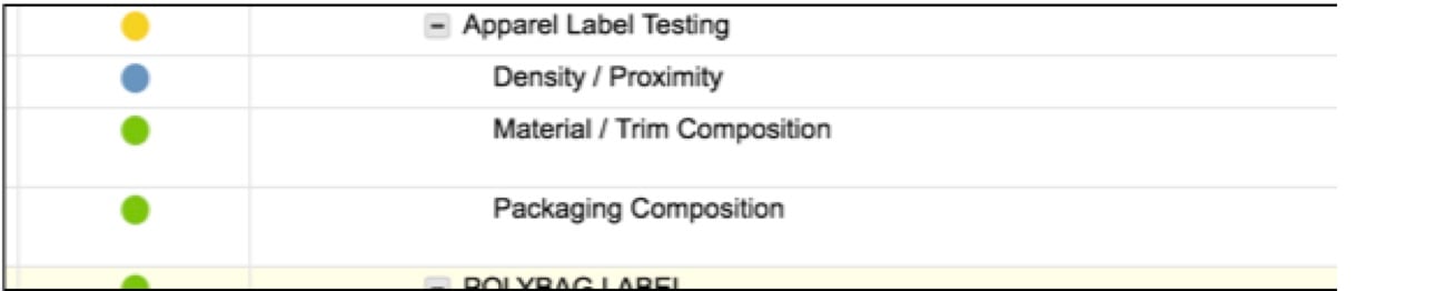
I am looking for the parent row to reflect a rollup of child row status color (RYG) AND if ALL child rows are blue (complete), have the parent row blue. I'm almost there, however, in the screenshot example below, the parent task is yellow although the 3 child tasks are either green (on track) or blue (complete).
Since the formula weights the different colors (R=0, Y=1, G=2) and divides the sum by the total number of child rows, the blue (completed) rows are counting against us in our average calculations.
Is there a way to re-write the formula to exclude blue rows from the average calculation?
=IFERROR(IF((COUNTIF(CHILDREN(), "Blue")) = COUNT(CHILDREN()), "Blue", IF((COUNTIF(CHILDREN(), "Yellow") + (COUNTIF(CHILDREN(), "Green") * 2)) / COUNT(CHILDREN()) <= 0.5, "Red", IF((COUNTIF(CHILDREN(), "Yellow") + (COUNTIF(CHILDREN(), "Green") * 2)) / COUNT(CHILDREN()) <= 1.5, "Yellow", IF((COUNTIF(CHILDREN(), "Yellow") + (COUNTIF(CHILDREN(), "Green") * 2)) / COUNT(CHILDREN()) <= 2.5, "Green")))), "-")
Comments
-
Yes. You just need to get the count of the blue children and subtract from the count of the children when setting your count for the IF statements.
..........(COUNTIF(CHILDREN(), "Green") * 2)) / (COUNT(CHILDREN()) - COUNTIF(CHILDREN(), "Blue")) <= 0.5, "Red".................
-
So helpful - thank you! I am now noticing that if the status color for the child rows are BLANK, then the parent will still turn blue (I would rather have it "-" or something). Do you have a recommendation to fix that?
Here is the latest formula:
=IFERROR(IF((COUNTIF(CHILDREN(), "Blue")) = COUNT(CHILDREN()), "Blue", IF((COUNTIF(CHILDREN(), "Yellow") + (COUNTIF(CHILDREN(), "Green") * 2)) / (COUNT(CHILDREN()) - COUNTIF(CHILDREN(), "Blue")) <= 0.5, "Red", IF((COUNTIF(CHILDREN(), "Yellow") + (COUNTIF(CHILDREN(), "Green") * 2)) / (COUNT(CHILDREN()) - COUNTIF(CHILDREN(), "Blue")) <= 1.5, "Yellow", IF((COUNTIF(CHILDREN(), "Yellow") + (COUNTIF(CHILDREN(), "Green") * 2)) / (COUNT(CHILDREN()) - COUNTIF(CHILDREN(), "Blue")) <= 2.5, "Green")))), "-")

-
If all children are blank, then the count will be 0. So if you incorporate in there somewhere...
IF(COUNT(CHILDREN()) = 0, "-", ..........
Another option would be to add the criteria to the third portion of your last IF statement.
............IF((COUNTIF(CHILDREN(), "Yellow") + (COUNTIF(CHILDREN(), "Green") * 2)) / (COUNT(CHILDREN()) - COUNTIF(CHILDREN(), "Blue")) <= 2.5, "Green", "-")))), "-")
-
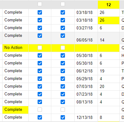
So what if your children are numbers that you want to average but you want to exclude rows where there is no value from the row count so it doesn't skew the average, but you need the row there chronologically?
This is the formula I was trying to use but it's not working
=(SUM(CHILDREN() / (COUNTIF(CHILDREN(), >=0))))
-
You could use something along the lines of
COUNTIFS(CHILDREN(), ISNUMBER(@cell))
This will only count children rows that have a number, so it will exclude text and blanks.


Help Article Resources
Categories
- All Categories
- 14 Welcome to the Community
- 10.7K Get Help
- 63 Global Discussions
- 69 Industry Talk
- 385 Announcements
- 3.5K Ideas & Feature Requests
- 55 Brandfolder
- 125 Just for fun
- 50 Community Job Board
- 464 Show & Tell
- 40 Member Spotlight
- 44 Power Your Process
- 28 Sponsor X
- 234 Events
- 7.3K Forum Archives
Check out the Formula Handbook template!