VLOOKUP for a range of numbers

raf45678 · 11/27/19

Hi Community,

I am looking to try and do a VLOOKUP against a range of numbers versus a single value. The function as I know it today only allows you to look up a value and pull the corresponding value for it (i.e., If the color is Green, then put 2 or if the color is Red, then put the number 3)

In my use case, I am looking at the difference between a start and end date of a project which is a number and then comparing that number to see if resides in a range and giving it a score

Example: The difference between 11/1/2019 and 2/22/2020 is 113 days. Knowing it is now 113, I want to compute that if its between 0-99 give me the value 1, 100-199 give me the value 2, etc.)

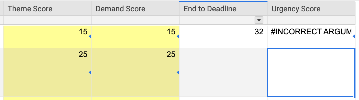
I can do this in Excel by referencing a table array and specific column of the score, but in SmartSheet I can't seem to look at more than 2 columns at a given time without getting a #INCORRECT ARGUMENT error

Any suggestions?

Samples of what I have attached. In this case, I would hope to get a value of 13 as 32 is between 0-179.

Screen Shot 2019-11-27 at 10.04.35 AM.png

Screen Shot 2019-11-27 at 10.04.42 AM.png

Mike Wilday · 11/27/19

Could you please provide the formula you have attempted to use there? It will help us help you troubleshoot.

raf45678 · 11/27/19

Hi Mike,

Here is the formula I am currently using: =VLOOKUP([End to Deadline]1, {ETX Solution Scoring Weights Range 4}, 3, false)

Where...

[End to Deadline]1 = the difference between two dates using the following formula: =NETDAYS([End Date]1, [Deadline Date]1)

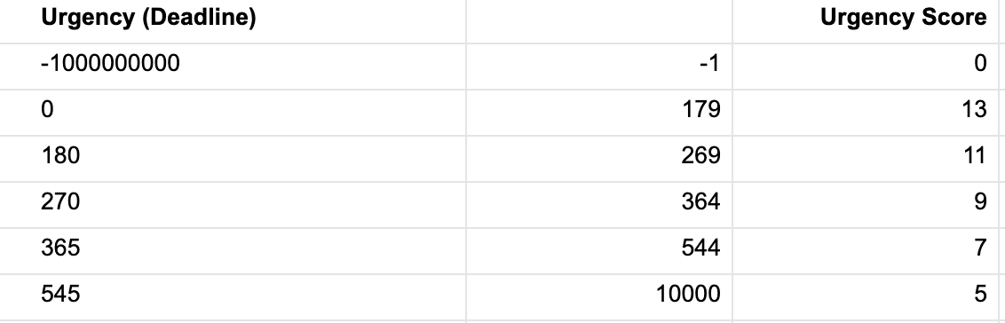
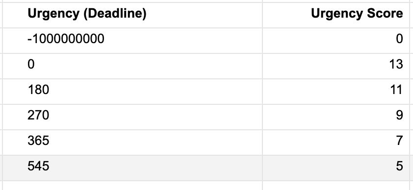
{ETX Solution Scoring Weights Range 4} = Reference to another sheet, the 2nd screenshot in my post

3 = column 3 where the scoring weights exist

true/false = neither appear to make a difference, but I would imagine false is the correct flag as I am not looking for an exact match

Mike Wilday · 11/27/19

Hmmm. I would try recreating your cross-sheet reference and ensure you are selecting all three columns.

Here is more on the error: https://help.smartsheet.com/articles/2476176-formula-error-messages#incorrectargumentset

And you'll actually want to use true which produces the approximate match.

https://help.smartsheet.com/function/vlookup

Paul Newcome · 11/27/19

I would suggest an INDEX/MATCH instead using a MIN/COLLECT to determine the row number.

It would look something like this...

=INDEX({Column to pull from}, MATCH(MIN(COLLECT({Reference Number Column}, {Reference Number Column}, @cell >= [End to Deadline]1)), {Reference Number Column, 0))

.

The MIN/COLLECT will pull the lowest number from the column containing your ranges that is greater than or equal to whatever is in your [End to Deadline]1 cell.

It will then use this number to match against to produce a row number for your INDEX function.

.

So using your example of 32, the MIN/COLLECT would pull the number 179 since that is the lowest number in the range that is higher than or equal to 32.

It will then use 179 as the value to search for in your range that contains those numbers.

The MATCH will hit on the number 179 in the range which will produce a number that will be used as the row number in your INDEX function.

.

Hope that makes sense.

raf45678 · 11/27/19

Thank you Mike and Paul. I will play more with the INDEX/MATCH functions as well as read up more on the error and see if I can create a simpler example to test with.

Will report back on what results I get and if they are successful or not.

Have a great Thanksgiving/Holiday if you are taking time off

raf45678 · 11/27/19

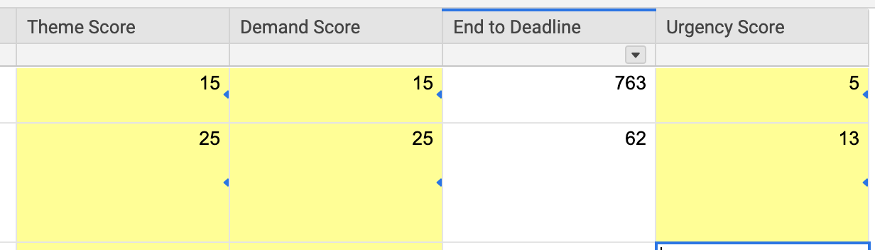
UPDATE: I think I resolved this! With a little playing around with the INDEX and MATCH functions I got the following results using the below formula:

=INDEX({ETX Solution Scoring Weights Range 7}, MATCH([End to Deadline]1, {ETX Solution Scoring Weights Range 8}))

Range 7 = The score I wanted to correlate with the number of days between two dates

MATCH (x,y) =

x = the value I was testing (32 in my previous example, but now its 763 for testing purposes)

y = the range of numbers to look up for correlation in my INDEX result

Still trying to understand what I built with this formula, but a little playing around goes a long way

Thank you guys for the feedback and help with this!

Screen Shot 2019-11-27 at 3.34.58 PM.png

Screen Shot 2019-11-27 at 3.35.14 PM.png

VLOOKUP for a range of numbers

Comments

Help Article Resources

Categories