Counting Instances Across Sheets
Answers
-
I'm not sure I understand. First you said...
"The Modality(Helper) correctly counted two BL masters for the same course as two separate BL masters:"
but then you go on to say...
"the Modality(Helper) formula counts its as two, when it should be one."
Are you able to show a screenshot of that specific section of the sheet?
-
Sorry about that. Yes, the formula does what it is supposed to do. It counts both BL masters. The Modality(Helper) cells BL-6w/BL-10w/OL-6w. This is "correct".
However, I don't want it to count both BL. I would prefer it to count as 1 blended, 1 online. If it doesn't it says there are a total of, say, 12 BL, 12 OL, and 12 BLO/OL, but there are only 11 required courses, so the percentage with each type of master completed is 114%.
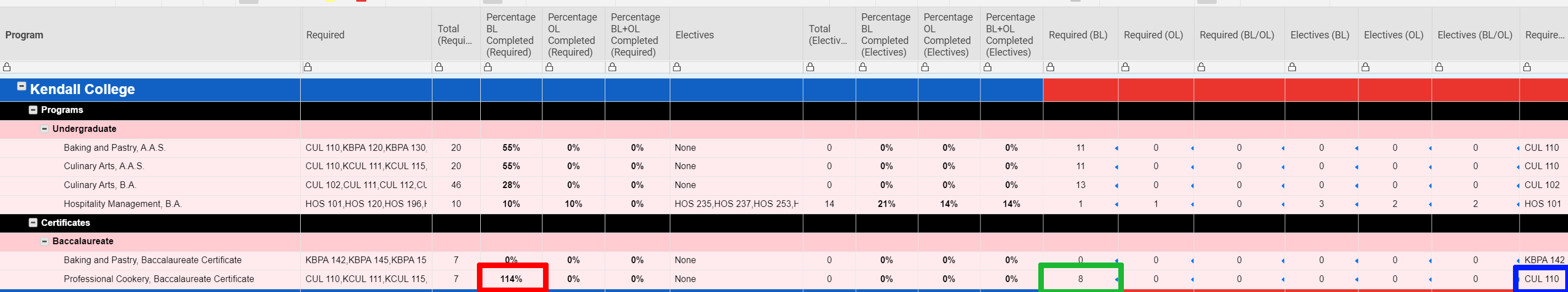
See the percentage (see red outline) is over 100% because the # of BL masters is 8 (see green outline) even though there are only 7 required courses. This happens becauses one of the required courses (see blue outline) has two OG (or BL) masters.
In the Kendall College course list sheet, see what shows in the Modality (Helper) column:
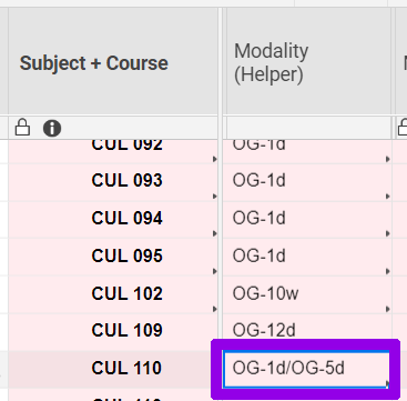
I adjusted your awesome formulas for OG (since in this college they don't have BL, blended, courses, they have fully on-ground or OG courses). For CUL 110, the same course, CUL 110, meets either for 1 day or 5 days, both on-ground.
I just want it to count 1 OG master for this course, not two, so the percentage (# of OG masters divided by number of required courses) is no more than 100%.
Is there a way around this? That is, when it counts how many required or elective courses in a program have a completed BL (or OL) master, when it looks at Modality(Helper), it only counts either modality once, rather than twice (if there happens to be more than one version of a BL or OL master)?
So, something like, if it contains "BL", add once, not for each BL that is in Modality(Helper)?
-
How about this...
Can you place both sheets in a folder then save a copy of the folder (this keeps links in place). Next... Remove/replace sensitive/confidential data. Then publish both sheets as "Edit by anyone" and share those links here?
This will allow me to see the data that is missing from your screenshots such as the full list in the [Required] field, all of the parsed columns, and the remaining Cull 110 rows that aren't shown in the second screenshot.
The formulas should actually NOT be counting the purple cell twice as it should only be counting cells where the [Modality Helper] contains "OG". The rows that aren't shown in your second screenshot should be blank in the [Modality Helper] column.
-
I can try to do the copies as you recommended.
I checked the required courses for this program. It requires the following courses:
CUL 110,KCUL 111,KCUL 115,KCUL 120,KCUL 121,KCUL 125,KCUL 127
The # of BL masters should be 5:
CUL 110 has "OG-1d/OG-5d" in Modality(Helper)
KCUL 111 has "OG-20d"
KCUL 115 has "OG-5d"
KCUL 120 has "OG-10d"
KCUL 121 has nothing (since none are completed)
KCUL 125 has "OG-5d"
KCUL 127 has nothing
So, total courses with OG masters should be 5, not 8
I removed each required course, one at a time, to see how it affected the total. When I removed KCUL 111, it reduced the total from 8 to 6. When I tested KCUL 125, it did the same thing. (If I remove CUL 110, KCUL 115, KCL 120, it reduces the total by one. Obviously when I tested removing KCUL 121 or KCUL 127, the total didn't change (they have no OG masters).
So, for some reason, KCUL 111 and KCUL 125 are counting twice.

-
It shouldn't be counting twice considering there is only one entry for each. That's odd. You may want to go ahead and also reach out to support. You may need a "back-end refresh" on the sheet because that seems a little "buggy". In the mean time... Try the following:
Log out
Clear cookies and cache
Log back in
-
@Paul Newcome - I need to parse out a multi contact list column. I have been following your parsing formula in this thread but I am having some difficulty. Here is my scenario- 2021 Bonus Goals can be shared. In the event they are shared, I need to create a row for each person the goal is shared with in the Bonus Goal Sheet. Using dynamic view, each person has to see their own shared goal and their weighting. I hope that is clear. In my scenario, I have Shared 1 and Shared 2 working but can't get Shared 3 and Shared 4 to work. They give the results of Shared 1. I am not sure what I am missing.
I am attaching a snap shot showing the column I am working with. I get the same results if I use the contact field or a text field. Below is the formula for Shared 4.
=IF($[Shared With Count]@row < 4, "", IFERROR(LEFT(SUBSTITUTE($[Shared With Text]@row + ",", JOIN($[Shared 1]@row:[Shared 3]@row, ",") + ",", ""), FIND(",", SUBSTITUTE($[Shared With Text]4 + ",", JOIN($[Shared 1]@row:[Shared 3]@row, ",") + ",", "")) - 1), ""))
Any help you can provide would be greatly appreciated.
Thanks,
Lynette
-
@LynnS25 The first thing I see right off would be that your formula is using "," (comma) as a delimiter, but your text field is using a ", " (comma space) as a delimiter. Try adjusting one of those so that they match and see if that clears up the issue.
-
@Paul Newcome - If I could hug you, I would! That was it. I think I looked at it for too many hours. Thank you so much.
-
@LynnS25 Happy to help. 👍️
-
Does this solution work if the Multi-Select Column is a Contact column? I am trying to use it, and it works for the first contact in the cell, and it works for the second, but then the third it just returns the first contact.
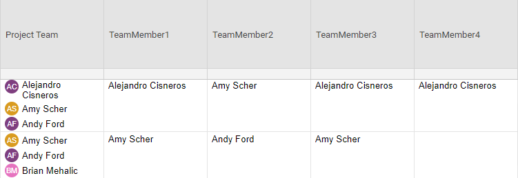
Formula in Column:
TeamMember1: =LEFT([Project Team]@row, FIND(",", [Project Team]@row) - 1)
TeamMember2: =IFERROR(LEFT(SUBSTITUTE($[Project Team]@row + ",", JOIN($[TeamMember1]@row:[TeamMember1]@row, ",") + ",", ""), FIND(",", SUBSTITUTE($[Project Team]@row + ",", JOIN($[TeamMember1]@row:[TeamMember1]@row, ",") + ",", "")) - 1), "")
TeamMember3 (etc.): =IFERROR(LEFT(SUBSTITUTE($[Project Team]@row + ",", JOIN($[TeamMember1]@row:[TeamMember2]@row, ",") + ",", ""), FIND(",", SUBSTITUTE($[Project Team]@row + ",", JOIN($[TeamMember1]@row:[TeamMember2]@row, ",") + ",", "")) - 1), "")
Am I doing something wrong? Or is it because the MultiS-Select Column is a contact column?
Thanks!
-
@Erin Ballantine Try adding a space after the comma in the delimiter.
So instead of
","
try
", "
That is the built in delimiter for multi-select contact columns.
-
EDIT: It seems as though instead of "', " or "," it prefers CHAR(10)
Would this also work on a list of items from a multiselect list?
The equation returns #invalid value on the destination column, it is selected as a text/number column
The information in the multiselect cell were transferred from another sheet via an automation function
-
@Delaram Hekmat The delimiter is going to depend on the type of column and the type of data that you are referencing.
In a contact type column, the delimiter is ", ". In a multi-select dropdown type column the delimiter is CHAR(10).
The reason for the error is going to depend on the exact formula that you are using, but I have a feeling it is going to depend on what you are using as your delimiter in the formula vs what the delimiter is that is being stored in the referenced cell. Even if it is in a multi-select dropdown, the delimiter could be different depending on the source of that data since you say it is coming from another sheet.
-
@Paul Newcome Hi Paul, hopefully you can help. I am trying to do something similar to the above, using the formula
=IFERROR(LEFT(SUBSTITUTE($[Technician Assigned]@row + ", ", JOIN($[Tech 1]@row:[Tech 3]@row, ", ") + ", ", ""), FIND(", ", SUBSTITUTE($[Technician Assigned]@row + ", ", JOIN($[Tech 1]@row:[Tech 3]@row, ", ") + ", ", "")) - 1), "")
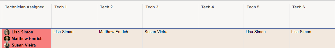
Anything beyond the number of assigned people + 1 (which ranges between 2 people and 6), It lists everyone after as the first person in the list. Is there anyway to fix this?
-
I figured it out, added if the cell before is not blank
=IF([Tech 1]@row <> "", IFERROR(LEFT(SUBSTITUTE($[Technician Assigned]@row + ", ", JOIN($[Tech 1]@row:[Tech 1]@row, ", ") + ", ", ""), FIND(", ", SUBSTITUTE($[Technician Assigned]@row + ", ", JOIN($[Tech 1]@row:[Tech 1]@row, ", ") + ", ", "")) - 1), ""))


Help Article Resources
Categories
- All Categories
- 14 Welcome to the Community
- 10.7K Get Help
- 63 Global Discussions
- 68 Industry Talk
- 385 Announcements
- 3.5K Ideas & Feature Requests
- 55 Brandfolder
- 125 Just for fun
- 50 Community Job Board
- 464 Show & Tell
- 40 Member Spotlight
- 44 Power Your Process
- 28 Sponsor X
- 234 Events
- 7.3K Forum Archives
Check out the Formula Handbook template!