Calculating cumulative values and reducing the total sum each day

Hi, I have a Safety Violation Sheet that uses Form Entry to record violations and assign a measured Probation Period in days. If there are multiple entries for an individual, the probation days should accumulate, at the same time the value reduces by (1) for each day that passes without incident.
I have (1) sheet that acts as a Name database for the company, and a column on that sheet that uses: =SUMIF({Safety Violation (Responses) Range 1}, [EMPLOYEE NAME]@row, {Safety Violation (Responses) Range 2}) to show the cumulative Probation Days accrued.
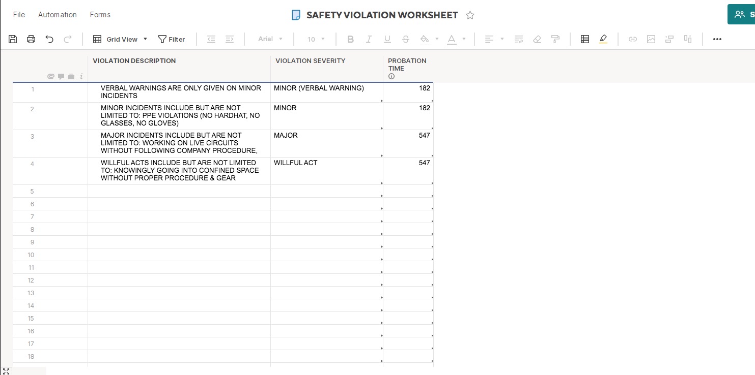
I also have a column on my Safety Violation Sheet that looks up the amount of days per violation entered: =VLOOKUP([Severity of Violation]@row, {SAFETY VIOLATION WORKSHEET Range 2}, 2, false)
and another column that reduces the Probation Period by (1) for each day that passes: =SUM(TODAY() - Timestamp@row) and =SUM([PROBATION END (HELPER)]@row - [PROBATION DAYS (HELPER)]@row)
Unfortunately the way I have the formula it reduces (1) day for each entry, so if John has (3) violations, (3) days are removed for each day that passes, and it should only reduce by (1) day for whatever has accumulated.
It seems I may need to move my Reduce by (1) day formula to my Name Database sheet, next to the the SUMIFS formula, but I'm having trouble with what that would look like.
I feel like there should be an easier way to do this...
Any help would be appreciated
Thanks!
Answers
-
Hello @Shawn Leahy
Hope all is well! Thank you for the description! May you please provide us screenshots (please block out any sensitive data) so we can try to replicate your setup to further test on this. Thank you~
Cheers,
Krissia
-
Hi Krissia,
Sure doing well and hope the same for you! Thanks for your response, hope you can help.
Here are a few screenshots, I cropped, hid, and redacted but hopefully left you enough to see what I am doing. I overlaid the formulas I am using in the columns they are in. Let me know if you need to see anything else.


-
To pull the most recent date for someone, you are going to want something along the lines of...
=DATEONLY(MAX(COLLECT({Source Data Timestamp Column}, {Source Data Name Column}, @cell = [Violator Name]@row)))
Subtracting that date from TODAY will give you how many days have passed since the last incident for that person.
=TODAY() - DATEONLY(MAX(COLLECT({Source Data Timestamp Column}, {Source Data Name Column}, @cell = [Violator Name]@row)))
-
Hi Paul,
Thanks for your time on this!
Those suggestions would work fine if we were only looking at the current Violation. Our program is cumulative to a point where a specific number results in Disciplinary Action, it does not reset with the newest violation.
What I am hoping for is to keep track of how many Probation Days that a Violator has accumulated and subtract days go by without incident, so:
Steve had a violation that cost him 182 Probation Days on June 1st, and another incident on July 13th that cost him 182 Probation Days. How many days does he have left as of August 4th?
(43) days passed between June 1 & July 13, and (20) days have passed between July 13th & August 4th
182 - 43 + 182 - 20 = 301 Probation Days Remaining as of August 4th.
The problem I am having is I don't have a method to Only subtract (1) Probation Day from someone that has multiple violations. It seems like I might need to prioritize the most recent Violation for a specific person and reduce that by (1) every day, but then somehow freeze all the others so they don't count down until the most recent zeros out... just not sure what that would look like.
Hope this is making sense.
Appreciate any help you can offer.
Thanks!
-
My apologies. I thought you had the other parts figured out all except for how many days since the last violation. I am going to have to get back to you when I have a little more time to work on this.
-
No worries, appreciate your time!
-
I think that, at each incident, you need to count the days since the last incident. In order to do that you need to figure out the MAX incident date among all incident dates that are less that this incident.
There is a thread right here with two published sheets that do this. I feel like the solution can be found down that path somewhere.
-
Hi James,
Appreciate your input on this, things had gotten quiet here and it seemed like this might have been too much to formulate.
I took a look at the examples you shared and I am not seeing an immediate solution to my issue, but you have at least you have given me some different ways to look at it.
I will run some more tests and see if I can get this to work.
Thanks!
-
@Shawn Leahy @James Keuning @Paul Newcome
Looked like a good challenge, what do you think of this.
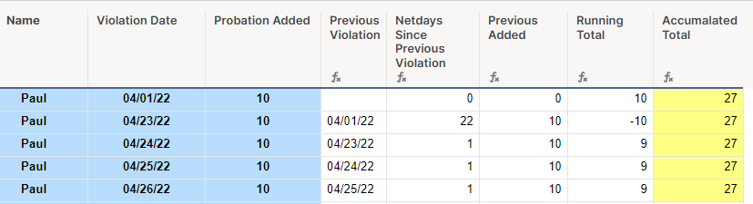
Previous Violation
=MAX(COLLECT([Violation Date]:[Violation Date], [Violation Date]:[Violation Date], MAX(COLLECT([Violation Date]:[Violation Date], Name:Name, Name@row, [Violation Date]:[Violation Date], <[Violation Date]@row), Name:Name, Name@row)))
Netdays since Previous Violation
=IFERROR(NETDAYS([Previous Violation]@row, [Violation Date]@row) - 1, 0)
Previously Added
=MAX(COLLECT([Probation Added]:[Probation Added], [Violation Date]:[Violation Date], MAX(COLLECT([Violation Date]:[Violation Date], Name:Name, Name@row, [Violation Date]:[Violation Date], <[Violation Date]@row), Name:Name, Name@row)))
Running Total
=IF(ISBLANK([Previous Violation]@row), [Probation Added]@row, IF([Previous Added]@row - [Netdays Since Previous Violation]@row < -[Previous Added]@row, -[Previous Added]@row, [Previous Added]@row - [Netdays Since Previous Violation]@row))
Accumulated Total
=SUMIF(Name:Name, Name@row, [Running Total]:[Running Total])
Edit
Added a second name to check, seems to be working

-
Hi Paul H,
Sorry for the delay in response, I have not had a lot of time to work in this and the bandaid I have in place is still holding...
Welcome to the string, and thanks for contributing!
This does seem to be working and it is a lot better than what I had, but I am still having a little trouble with the Accumulated Total. Your Model looks good if the "Probation Added" value stays the consistent. I noticed when I entered a NEW entry, the "Accumulated Total" populated before a value was entered in the "Probation Added" field, and adding a different value made no difference
Looks like with the "Running Total" sums the "Previous Added" less the "Netdays Since Previous Violation", but if the "Previous Violation" is blank it populates the "Probation Added" value at the row. This kinda works, but it is not looking at the current Violation, which could be higher and cause for suspension (any value higher than 547 probation days results in suspension, so I need to be looking at the current Probation Added).
It also looks like the relevance in time is only to the previous violation, so if an employee has a few violations within a few months it calculates pretty well, but if the worker goes a few years before he get's another incident it does not accurately reduce the days that have past. It looks like when the new violation is entered the formula sums the value of the previous "Previous Added" if the "Netdays Since Violation" is less than the value in "Previously Added", but it will subtract, but no more than that value ("PA"=182, "NSPV"=172, "RT"=10) ("PA"=182, "NSPV"=760, "RT"=-182), and the "Running Total" holds all the previous data from years past that have not rolled off.
The intent is fairly simple: Start with (0) "Probation Days" and add in violations as they are issued, and each day that passes without incident reduces the accumulated total by (1). If you reach (547) Probation Day, you are terminated. Unfortunately it is proving a bit more difficult to build a formula to calculate correctly.
I think James is right, the answer is in here somewhere.
Appreciate your help with this!


Help Article Resources
Categories
- All Categories
- 14 Welcome to the Community
- 10.6K Get Help
- 63 Global Discussions
- 67 Industry Talk
- 385 Announcements
- 3.5K Ideas & Feature Requests
- 55 Brandfolder
- 125 Just for fun
- 50 Community Job Board
- 464 Show & Tell
- 40 Member Spotlight
- 44 Power Your Process
- 28 Sponsor X
- 234 Events
- 7.3K Forum Archives
Check out the Formula Handbook template!