Formula help

Hello, I am trying to do a vlookup on my smartsheet task list to reference a different smartsheet which looks up for example "312" returns the value two columns over, which is a date, and then minus 90 days from that date and returns that date in the cell. Is there a way to do this?
Comments
-
=(VLOOKUP([Column Name]@row, {Reference Sheet Range 1}, 3) - 90)
For the reference sheet range, you would start with the leftmost column being the one containing the 312 and the rightmost column being the date.
The 3 in the formula is the column number of the data you want to pull from your table with the leftmost column being 1.
From there simply subtract 90, and you're all set. Just make sure the target column (the one where you have the formula) is a Date type column.
-
Thank you! My formula is returning no match when there is a match. can you please help?
The value I am looking up is column 38 row 6, referencing the date column in sheet 2.
=(VLOOKUP([Column38]6, {date}, 9) - 90)
-
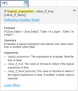
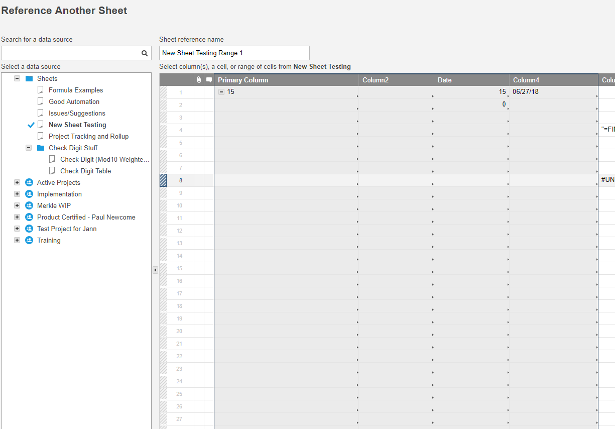
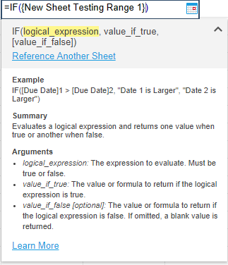
When you reference another sheet, the easiest way is to use the "Reference Another Sheet" link in the formula help box. Select your range from there and click "Insert Reference
Based on the second image below I would use 4 as my column reference after the sheet reference denoting that it is the 4th column in the RANGE, not necessarily the 4th column in the sheet.

Help Article Resources
Categories
- All Categories
- 14 Welcome to the Community
- 10.7K Get Help
- 63 Global Discussions
- 69 Industry Talk
- 385 Announcements
- 3.5K Ideas & Feature Requests
- 55 Brandfolder
- 125 Just for fun
- 50 Community Job Board
- 464 Show & Tell
- 40 Member Spotlight
- 44 Power Your Process
- 28 Sponsor X
- 234 Events
- 7.3K Forum Archives
Check out the Formula Handbook template!