Welcome to the Smartsheet Forum Archives
The posts in this forum are no longer monitored for accuracy and their content may no longer be current. If there's a discussion here that interests you and you'd like to find (or create) a more current version, please Visit the Current Forums.
Sum of column items respecting the filter

Hi all,
I've started using Smartsheet recently, so I am sorry if this is a newbie question ![]() I've tried to search for a solution, but nothing specific about this came up.
I've tried to search for a solution, but nothing specific about this came up.
Anyway, I got the column SUM as open-ended, summing all rows correctly.
But when I enable a filter, for example only seeing rows in last 60 days, the sum amount remains the same. I understand that the columns are only hidden while the filter is active, so the SUM formula always counts on them.
Let me know if there is a way to go around this and how, I would like the SUM to be 'dynamic' showing me only the amount of rows I have visible.
a great software btw!
thanks in advance
Deckey
Comments
-
Hi Deckey, there are a couple options.
The first, is to apply the filter, highlight the cells you want to SUM and look at the bottom right of your screen. There are automatic formulas that can perform quick calculations for you.
Another option is to use a SUMIF which can sum a group of cells if they meet a certain criteria.
Check out our Help Center article on formulas for help setting this up: http://help.smartsheet.com/customer/en/portal/articles/775363-using-formulas
-
Hi Travis, thanks for the input.
I've made a workaround using SUMIF as you suggested, by inserting a column 'Include' checkbox as a criteria.
So, after applying the filter to show only relevant rows, I can 'check' the ones I want to show in a summary.
thanks again,
Deckey
-
this seems like an awkward work around and frankly not really that dynamix. I kind of defeats the whole purpose of the filter if you still need to go back and check them all off.
Are there any other possible solutions. Seems like this is a function that would be pretty desirable across a wide range of users.
-
Peter, it would depend on the type of data you want to SUM. A lot of data can be included in a SUMIF without the need for a checkbox column. For example, "sum every cell in X column where Y column cell is John". Only more complex scenarios such as, "sum every cell in X column where Y column cell date is between these two dates", would require a third column such as a checkbox.
What type of data are you trying to SUM?
-
I was able to accomplish a pretty intuitive means in which to accomplish the OP's intent through some formula trickery and an intentional SS layout. The context of this dialog is with a running ledger of multiple Project's and Exercise's orders on a given Program, with tracking of booked projects, invoices, receipts, and costs.
A graphical image referenced in the following is available here: http://i.imgur.com/icw0dyw.png
The SS is structured with a typical running ledger, with row 2 being the top-level parent. This is intentional, as row 1 is the 'query' row (green arrow). When either or both of the two 'query' cells (red circle) is selected, formulas serve to provide subtotals and relevant information to the right of the Project/Exercise dropdowns (in the row 1 cells in the red square).
To make use of this query row, I first select the desired parameters in either of the Project1 and Exercise1 cells (or both, if higher fidelity filtering needed - Orange Arrow in Red Circle) and then apply SS Column Filters to match that which I selected in the dropdows (Blue Arrow - filters selected without parent rows being displayed).
The results, once the SS Column Filters is applied, is depicted here: http://i.imgur.com/LzMTtEi.png
The results of the filtering is presented below the summary row, which provides the subtotals of only the filtered data presented. Misson Accomplished.
A side benefit is that a simple 'Project'/'Exercise' fiscal health check can be made by just selecting the dropdownss in Row1 (Project1, Exercise1). This enables the PM to quickly assess the fiscal parameters on an overall project basis, as well as for each exercise therein (without having to apply filters). And, the Grand Total Parent Row on the unfiltered SS serves to give a quick fiscal health check across the whole of the Program, inclusive of all Projects/Exercises.
So, to help with replicating this, should someone desire to do so, I offer the following (error avoidance baked into the formulas a bit):
Doc_Ref_#1 (Percent invoiced text): =IF(AND(Project1 = "-", Exercise1 = "-"), "-", IF(OR(BOOKED1 = 0, BOOKED1 = ""), "No Booking", LEFT(ROUND(INVOICED1 / BOOKED1, 3) * 100, 4) + "% Invoiced"))
BOOKED1: =IF(AND($Project1 = "-", $Exercise1 = "-"), "-", IF(AND(OR($Project1 = "", $Project1 = "-"), OR($Exercise1 = "", $Exercise1 = "-")), "", IF(OR($Exercise1 = "", $Exercise1 = "-"), SUMIFS(BOOKED$2:BOOKED$344, $Project$2:$Project$344, $Project1), IF(OR($Project1 = "", $Project1 = "-"), SUMIFS(BOOKED$2:BOOKED$344, $Exercise$2:$Exercise$344, $Exercise1), SUMIFS(BOOKED$2:BOOKED$344, $Project$2:$Project$344, $Project1, $Exercise$2:$Exercise$344, $Exercise1)))))
INVOICED1: =IF(AND($Project1 = "-", $Exercise1 = "-"), "-", IF(AND(OR($Project1 = "", $Project1 = "-"), OR($Exercise1 = "", $Exercise1 = "-")), "", IF(OR($Exercise1 = "", $Exercise1 = "-"), SUMIFS(INVOICED$2:INVOICED$344, $Project$2:$Project$344, $Project1), IF(OR($Project1 = "", $Project1 = "-"), SUMIFS(INVOICED$2:INVOICED$344, $Exercise$2:$Exercise$344, $Exercise1), SUMIFS(INVOICED$2:INVOICED$344, $Project$2:$Project$344, $Project1, $Exercise$2:$Exercise$344, $Exercise1)))))
RECEIPTS1: =IF(AND($Project1 = "-", $Exercise1 = "-"), "-", IF(AND(OR($Project1 = "", $Project1 = "-"), OR($Exercise1 = "", $Exercise1 = "-")), "", IF(OR($Exercise1 = "", $Exercise1 = "-"), SUMIFS(RECEIPTS$2:RECEIPTS$344, $Project$2:$Project$344, $Project1), IF(OR($Project1 = "", $Project1 = "-"), SUMIFS(RECEIPTS$2:RECEIPTS$344, $Exercise$2:$Exercise$344, $Exercise1), SUMIFS(RECEIPTS$2:RECEIPTS$344, $Project$2:$Project$344, $Project1, $Exercise$2:$Exercise$344, $Exercise1)))))
COSTS1: =IF(AND($Project1 = "-", $Exercise1 = "-"), "-", IF(AND(OR($Project1 = "", $Project1 = "-"), OR($Exercise1 = "", $Exercise1 = "-")), "", IF(OR($Exercise1 = "", $Exercise1 = "-"), SUMIFS(COSTS$2:COSTS$344, $Project$2:$Project$344, $Project1), IF(OR($Project1 = "", $Project1 = "-"), SUMIFS(COSTS$2:COSTS$344, $Exercise$2:$Exercise$344, $Exercise1), SUMIFS(COSTS$2:COSTS$344, $Project$2:$Project$344, $Project1, $Exercise$2:$Exercise$344, $Exercise1)))))
COMMENTS1**: =IF(AND(Project1 = "-", Exercise1 = "-"), "-", IF(OR(INVOICED1 = 0, INVOICED1 = ""), "No Receivables", Nets1 + " Net | " + LEFT(ROUND((INVOICED1 - COSTS1) / INVOICED1, 3) * 100, 4) + "% Mar | " + LEFT(ROUND(RECEIPTS1 / INVOICED1, 3) * 100, 5) + "% Rcvd" + " | " + Nets2 + " Due"))
** And, for parsing a number to a string, I had to become a hack (as there may very well be a better way.?.) and use a series of hidden columns to do so, as I wanted readable monetary figures to be included in a cells contents as part of a built-up text string, and SS doesn't yet have a TEXT function that I could find (there is some error avoidance herein as well):
cent1: =IF(AND(Project1 = "-", Exercise1 = "-"), "-", IF(INT(INVOICED1 - COSTS1) = INVOICED1 - COSTS1, ".00", IF(INT((INVOICED1 - COSTS1) * 10) = (INVOICED1 - COSTS1) * 10, RIGHT(INVOICED1 - COSTS1, 2) + "0", RIGHT(ROUND(INVOICED1 - COSTS1, 2), 3))))
hund1: =IF(AND(Project1 = "-", Exercise1 = "-"), "-", RIGHT(INT((INVOICED1 - COSTS1) / 1), 3))
thous1: =IF(AND(Project1 = "-", Exercise1 = "-"), "-", IF(INVOICED1 - COSTS1 >= 1000, RIGHT(INT((INVOICED1 - COSTS1) / 1000), 3), ""))
mils1: =IF(AND(Project1 = "-", Exercise1 = "-"), "-", IF(INVOICED1 - COSTS1 >= 1000000, RIGHT(INT((INVOICED1 - COSTS1) / 1000000), 3), ""))
bils1: =IF(AND(Project1 = "-", Exercise1 = "-"), "-", IF(INVOICED1 - COSTS1 >= 1000000000, RIGHT(INT((INVOICED1 - COSTS1) / 1000000000), 3), ""))
trils1: =IF(AND(Project1 = "-", Exercise1 = "-"), "-", IF(INVOICED1 - COSTS1 >= 1000000000000, RIGHT(INT((INVOICED1 - COSTS1) / 1000000000000), 3), ""))
Nets1:
=IF(AND(Project1 = "-", Exercise1 = "-"), "-", IF(INVOICED1 - COSTS1 < 1000, "$" + hund1 + cent1, IF(INVOICED1 - COSTS1 < 1000000, "$" + thous1 + "," + hund1 + cent1, IF(INVOICED1 - COSTS1 < 1000000000, "$" + mils1 + "," + thous1 + "," + hund1 + cent1, IF(INVOICED1 - COSTS1 < 1000000000000, "$" + bils1 + "," + mils1 + "," + thous1 + "," + hund1 + cent1, IF(INVOICED1 - COSTS1 < 1000000000000000, "$" + trils1 + "," + bils1 + "," + mils1 + "," + thous1 + "," + hund1 + cent1, "UGH! See Tod"))))))
Oh, one last note, I had to hard-code the row limits in the formulas above (i.e. row2:row344). This is because of the fact that using this approach, the subtotaled data is in row1 and recursion-avoidance is required. It is a limitation I've become accustomed to both herein and well as with Excel, when making use of summary rows above columns of relevant data.
I'm sure that some will review this and twitch a bit, declaring it too Rube Goldberg-ish. I get it. It works for me (and the non-technical boss). For those who do endeavor to tackle this, I will try to answer any questions. No promises on timeliness, however, as I am pretty task saturated. Good luck.
-t
-
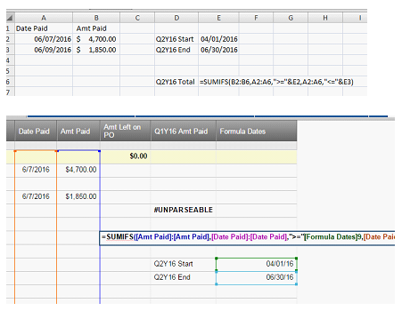
Can anyone tell me why this formula works in Excel, but the "&" breaks the formula in smartsheet?
-
Any update on this? Formulas should respect filters. This is a basic element of Excel's table total and frankly common sense. To have to write a complex sumifs formula defeats the simplicity of a filter.

Categories
- All Categories
- 14 Welcome to the Community
- 10.9K Get Help
- 65 Global Discussions
- 69 Industry Talk
- 385 Announcements
- 3.6K Ideas & Feature Requests
- 56 Brandfolder
- 125 Just for fun
- 50 Community Job Board
- 464 Show & Tell
- 40 Member Spotlight
- 44 Power Your Process
- 28 Sponsor X
- 234 Events
- 7.3K Forum Archives