Sumifs with Date Range

Have you tried factoring in the DAY function to try to pull a percentage of the month (almost like prorating which can also be done in SS)?

=DAY([End Date Column]@row) / DAY(DATE(YEAR([End Date Column]@row), MONTH([End Date Column]@row) + 1, 1) - 1)

This will give you a decimal (one day is approximately .035) based off of how much of the month was actually worked. You may be able to factor this in somehow to get more accurate counts.

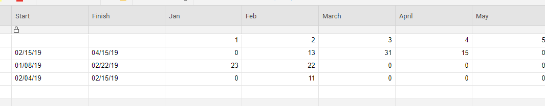
It is possible. I found the easiest way was to build a table as in the screenshot below. In the Jan2 cell, enter the following formula:

.

=IF(AND(Jan$1 = MONTH($Start@row), Jan$1 = MONTH($Finish@row)), DAY($Finish@row) - DAY($Start@row), IF(Jan$1 < MONTH($Start@row), 0, IF(MONTH($Start@row) = Jan$1, DAY(IFERROR(DATE(YEAR($Start@row), Jan$1 + 1, 1), DATE(YEAR($Start@row) + 1, 1, 1)) - 1) - DAY($Start@row), IF(AND(Jan$1 > MONTH($Start@row), Jan$1 < MONTH($Finish@row)), DAY(IFERROR(DATE(YEAR($Start@row), Jan$1 + 1, 1), DATE(YEAR($Start@row) + 1, 1, 1)) - 1), IF(Jan$1 = MONTH($Finish@row), DAY($Finish@row), IF(Jan$1 > MONTH($Finish@row), 0))))))

.

You can then dragfill across and down as needed. Here's a basic breakdown of what happens...

1. If the Start and Finish Months both equal the corresponding month column, it will just subtract the days and give you the difference. (Feb4)

2. If the Start Month is greater than the corresponding month column, it will display 0 to show that no days were worked in that month. (Jan2)

3. If the Start Month is the same as the corresponding month column, it will...

     3.a. Go to the First of the next month and then subtract a day. This ensures you will always be calculating from the proper number of days regardless of month. In the case of December (the IFERROR section), it will go to the first day of the first month of the next year and then subtract a day. 

     3.b. It will then subtract the starting day from the last day of the month to display how many days were worked in that first month. (Feb2)

4. If the corresponding month column is greater than the Start Month but less than the Finish Month, it will use a similar calculation as in step 2 to pull the last day of the month (meaning the entire month was worked). (March2)

5. If the Finish Month is the same as the corresponding month column, it will simply pull the day from the finish date as that will be how many days in that month were worked. (April2)

6. And finally... If the Finish Month is less than the corresponding month column, then there were no days worked in that month, and the formula will give you a 0. (May2)

Yes. How were you wanting it displayed? Something along the lines of...

.

Oct 18     Nov 18      Dec 18      Jan 19      Feb 19       March 19

.

or would you prefer to only show what was done in 2019 and have the 2018 data elsewhere? Maybe a 2018 table and a 2019 table and then compare the two to show overlap?

Take a glance at this mess. Here's a published link to the sheet (currently read only).

https://app.smartsheet.com/b/publish?EQBCT=4891ed355237415880f6d328ec44ad23

.

And here's the formula used (with column and row references locked to make dragfill/autofill work easily)

=IF(AND($Start@row >= DATE([Month 1]$2, [Month 1]$1, 1), $Finish@row <= IFERROR(DATE([Month 1]$2, [Month 1]$1 + 1, 1), DATE([Month 1]$2 + 1, 1, 1)) - 1), $Finish@row - $Start@row, IF(AND(MONTH($Start@row) = [Month 1]$1, YEAR($Start@row) = [Month 1]$2), (IFERROR(DATE([Month 1]$2, [Month 1]$1 + 1, 1), DATE([Month 1]$2 + 1, 1, 1)) - 1) - $Start@row, IF(AND($Start@row < DATE([Month 1]$2, [Month 1]$1, 1), $Finish@row > IFERROR(DATE([Month 1]$2, [Month 1]$1 + 1, 1), DATE([Month 1]$2 + 1, 1, 1)) - 1), DAY(IFERROR(DATE([Month 1]$2, [Month 1]$1 + 1, 1), DATE([Month 1]$2 + 1, 1, 1)) - 1), IF(AND(MONTH($Finish@row) = [Month 1]$1, YEAR($Finish@row) = [Month 1]$2), DAY($Finish@row)))))

.

To get the Total Days Worked, I used a basic 

=SUMIFS([Month 1]@row:[Month 36]@row, [Month 1]@row:[Month 36]@row, ISNUMBER(@cell))

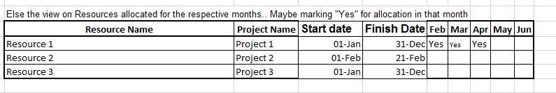
Thanks.. this is wonderful formula which helped me aswell. Though just wanted to check if we can get just an some value which will indicate that the FTE was allocated in that month.  

To explain.. Maybe the allocation is between Jan 2019 till Mar 2019... it should just Indicate "Y" for the allocated months - Jan, Feb and Mar. For Apr it can be blank row.

Thanks for the response Paul

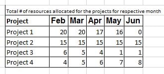
Actually looking for data as per the screenshot 1. this is just count of resources assigned on the project for the respective months. 

If the above is not possible then the screenshot 2 - which is indicating the resource allocation for the specific month. 

Thanks, though how can i count for the specific projects as in the screenshot 1.

I just want the total monthly resources count on the specific project.. month on month

Thank you for the response. I will try and get back to you..