Best Of
Re: May Question of the Month - Join the conversation and receive a badge
Thank you @Rebeca S. for the AMAZING question - you are pretty cool yourself by the way 😎
There are so many delicious things in the area as I am from Western PA (born and raised)/Eastern OH (where I currently live). This area is full of international influence from the Polish and Italians. I may need to make a 3-course meal for my community friends here (who would complain? I wouldn't!).
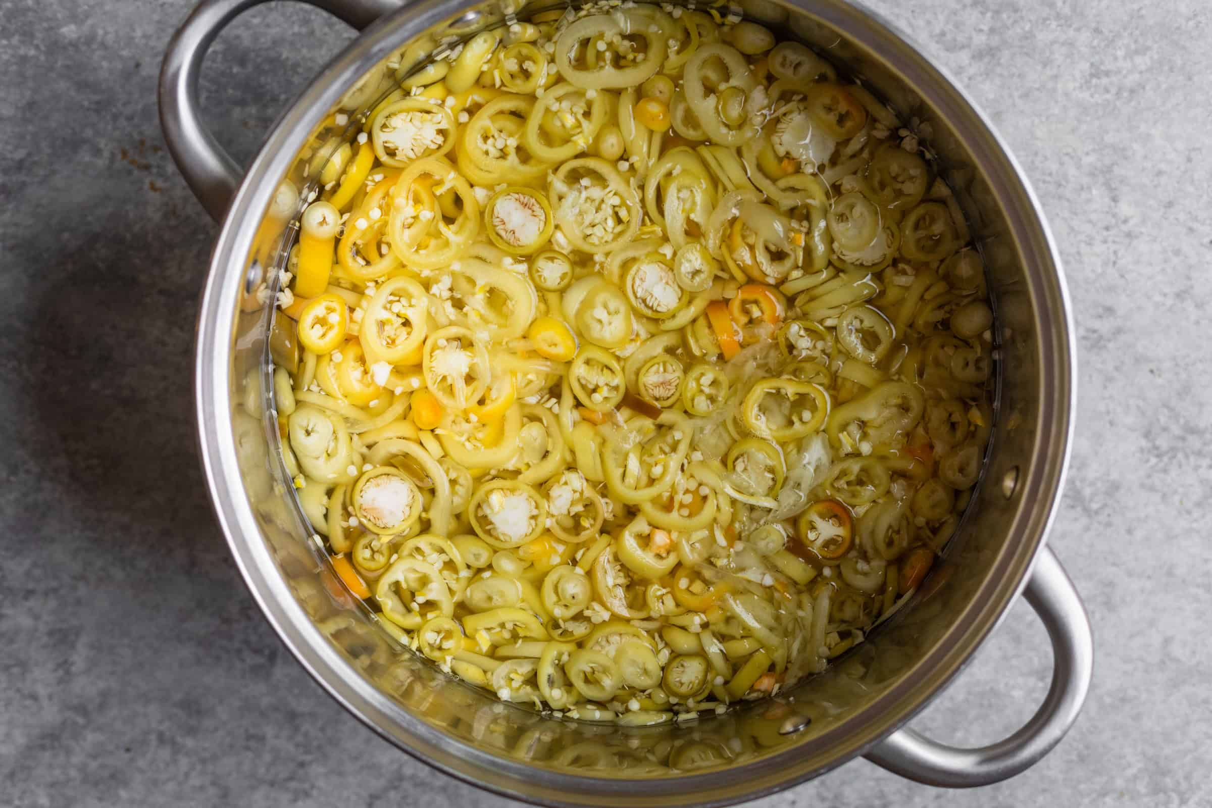
We'd start with some delicious peppers in oil and pita/naan bread. A delicious start - and sometimes sneaky kick - that makes your heart happy.
We'd then move into a good Primanti's Sandwich. Especially the Pittsburger (their #2 seller by the way, their #1 is 🍺), a long hamburger patty with provolone on the softest Mancini's Italian bread with Tomato, oil/vinegar-based slaw, and French fries. This sandwich is the perfect amount of sweet, salt, savory, vinegar, and crunch!
Then finally - last and CERTAINLY not least is the cookie table tradition. Where friends and family make cookies to share - normally at weddings - and come by the 1000s. I'll make you at least 3 kinds personally - lady fingers, buckeyes, and Hershey kiss blossoms. I'll make more if you tell me your favorite cookie - as I love learning new recipes.
 Akblevins
Re: May Question of the Month - Join the conversation and receive a badge
If visiting, I'd like you to come by in August and September when the wild blackberries are ripe. There is nothing sweeter than picking your own fruit, spending time chatting and enjoying the mild weather, taking them home and washing them to make into a sweet treat. They are 100% better than store-bought, and you can eat as you pick. And you pick as much as your bucket can carry since there ae bushes everywhere.
 AnemonePoppy
Re: May Question of the Month - Join the conversation and receive a badge
Mint Prawns
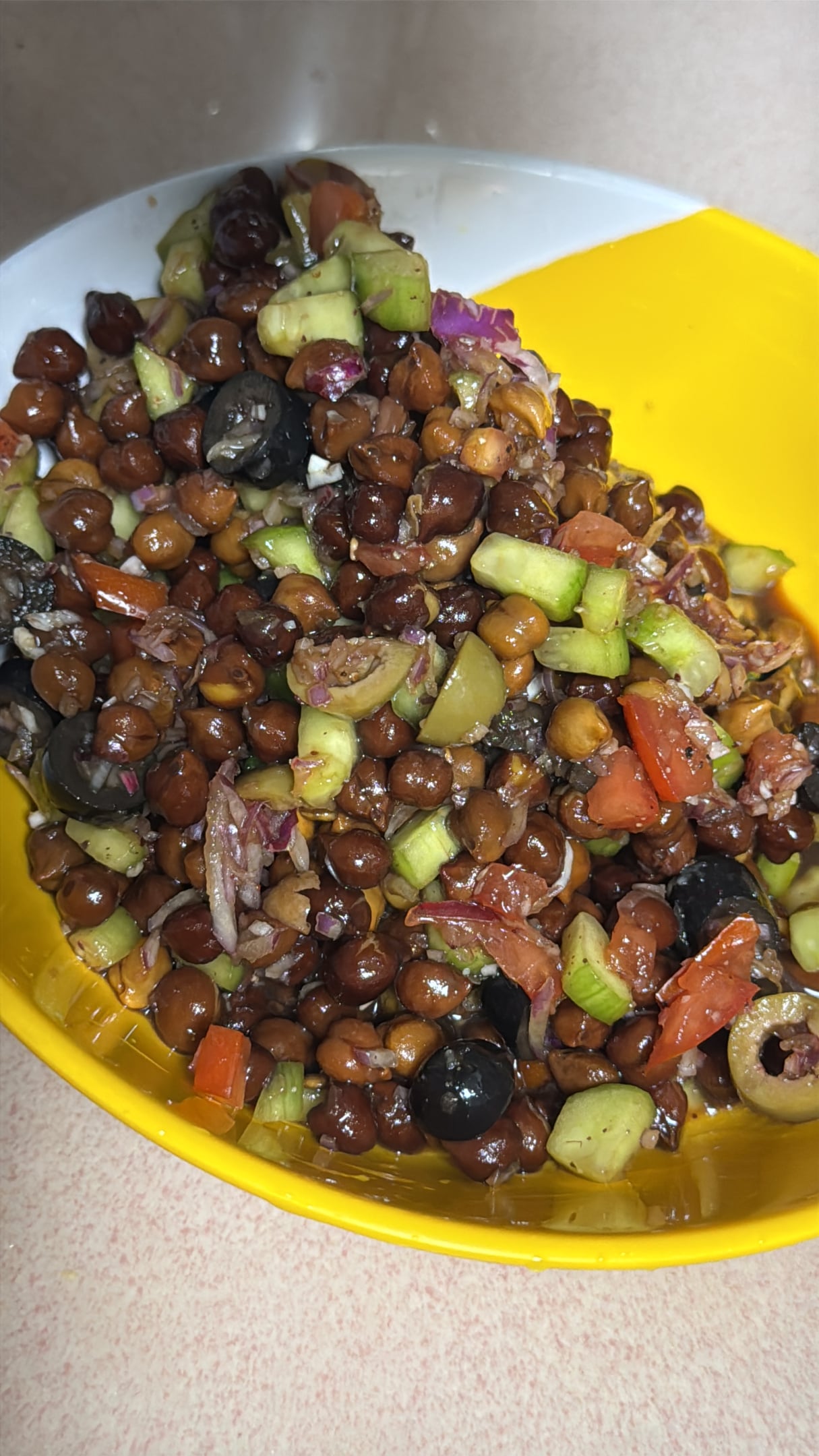
Healthy Salad
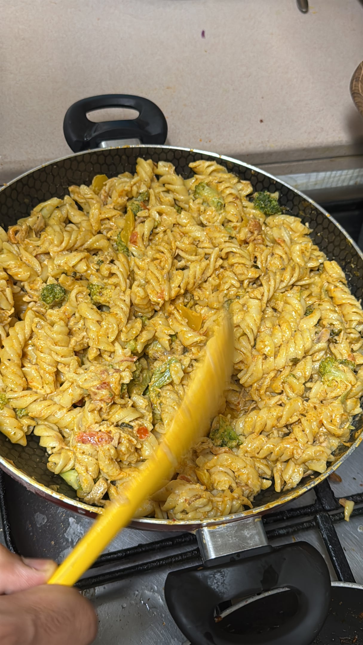
Broccoli Cheese Pasta
Cooked at Home
Re: May Question of the Month - Join the conversation and receive a badge
I must not be far from @Jesse G. Because I would serve them a Welsh. Don't worry, nothing cannibal about it, just bread and ham topped with melted cheddar and cooked with beer, that's my favourite dish from the north of France.
Re: May Question of the Month - Join the conversation and receive a badge
If I had to choose a place to take someone who was visiting it would definitely be Brooks Sandwich House. It's a small burger shack where you can eat outside at the tables or in your car in the lot cause it never makes it back home. Worth the standing in line.
 Shaq McWilliams
Community Corner Newsletter [May 2026]
Happy May, Community.
How is your 2026 so far? It’s still early, but I hope this year is shaping up to be a fantastic one for you! It’s certainly an exciting time for us here, and I want to share some of those fun updates with you: recent product releases, special shout outs, a new Community page, and — our brand new Community Events! Read on to learn all about that! 😃
📌 We post these newsletters every month to help you stay up to date. Give the previous edition a read if you haven’t yet so you don’t miss anything.
Community highlights
Help us welcome some of our newest Member introductions in Show & Tell or look through the Trending section for more ways to connect.
Say hello to these Community Members 👋🏻
You can find more new members and say hello here.
---
Recent Product Releases
- CLI Power Tools: Open-source Claude Code agents that turn Smartsheet's depth into your AI advantage
- Commenting and attachments now free for internal users with new CONTRIBUTOR seat type
- AI auto-fill makes mobile forms faster and easier to complete
- Full CRUD operations for reports now available on Public API
- Enterprise security features now available for Smartsheet Mobile App
- New in Data Shuttle: track rows processed and get deeper workflow details in your CSV report
What’s it going to be? Head to the Smartsheet Product and Ideas Topic to share and vote on ideas.
---
Community updates
In Case You Missed It (ICYMI)
Introducing Community Events 🎉
Discover virtual member-led events to bring your knowledge to the next level!
May Question of the Month
Join our food recommendations thread by May 31
[NEW] Smartsheet Advocacy Programs Page
Find the perfect opportunity for you!
---
Overachiever's Motivation Mix
The Smartsheet Overachievers are here to give you the songs that will keep you going and keep you achieving! Here’s what’s on the playlist right now.
PinkPantheress ft. Zara Larsson - Stateside
“Always rocking this when I'm on that Smartsheet grind or commuting in the morning to work!”
- Andrei Veloso ( @A.Veloso), Project Manager at Douglas Pharmaceuticals + Overachiever
---
Member Appreciation
See Activity feed for more
This month's leaderboard
Pass the mic 🎤 Community Champions
Community Champions are members who demonstrate generosity in sharing best practices and support with others on the platform.
“It means having a support system of fellow Champions and resources I can lean on. That’s what makes the Smartsheet Community truly special - you’re never alone. It’s such a stark contrast to other tools, and I’m genuinely grateful to be a part of something this supportive and collaborative!”
- @Cayla Davis , Global Technology Manager at Amex GBT (Read more about Cayla in her Member Spotlight)
Do you know someone in the Community who should be next month's Member Spotlight? Nominate them here.
---
Give us your feedback
Have ideas for the next Community Corner? Leave your thoughts in the comments!
Note: Unfollow this Topic if you'd no longer like to receive alerts. We'll miss you!
 Rebeca S.
Re: Can you use 2 match criterias in an index/match formula?
Another question I needed an answer to just now! Way to go @Paul Newcome
Re: Can you use 2 match criterias in an index/match formula?
It is possible using an INDEX/COLLECT.
=INDEX(COLLECT({range to pull from}, {first criteria range}, first criteria, {second criteria range}, second criteria), 1)
 Paul Newcome


