Best Of
Re: 🎉 Exciting News: The Smartsheet Architect Learning Path is Here!
@darkmatter To get the Certified Architect you have to have the Certified Professional qualification.
There are 2 parts an example and a portfolio of work submission and one exam. There is a marking guide for the submission. You would start work on preparing and collecting information for your portfolio now. If you feel you understand the concepts well (which I think you would based on what you have shared in the community) you could look at just paying the exam fee, but send email email to smartu@smartsheet.com to check if paying the exam fee lets you submit the portfolio of work/evidence and get graded.
Getting my portfolio ready is taking some time. You have to show evidence of all the skills with screen shots and training materials etc. They suggested you over document to ensure you pass. Redacting information on sheet shots is taking time too. You submit one pdf file of under 500 MB. (I hope you have Abode pro licence to pull it all together eg screen shots, word docs, SharePoint sites, PowerPoints).
Details on Certified Professional
Portfolio - Evidence Submission Template
Then you can look ahead to the Architect portfolio / evidence of work too
Details on Certified Architect
Portfolio - Architect Evidence Submission Template
I paid for the learning pass (covers all courses and 2 x exam attempts for both levels), but have found I didn't learn any new skills in the professional courses, just saw exams of what they wanted submitted for the portfolio.
The Troubleshooting Architecture course was teaching a process for correcting errors. No new skills learnt, but the process was good to be across if you have multiple builders/fixers/IT people supporting a solution and trying to fix things.
My next 2 courses are this week and next week. I will let you know what I think.
 Amy Munro
Re: What are some fun and unique ways you use Smartsheet?
I use Smartsheet to record milestones, memorable moments, and interactions with our 4-year-old son, who was recently diagnosed with Level 3 Autism Spectrum Disorder (ASD). Throughout the day, I log words or phrases he says using a form with category drop-down selections. The entries are automatically organised and displayed on a dashboard, making it easy to track his progress ❤️
This data becomes incredibly helpful in our bi-weekly speech therapy sessions and when meeting with his doctors. It gives our speech therapist a week-by-week picture of his progress, allowing her to tailor each session without needing a full rundown from us, so we can dive right into the lesson.
 Jay Mondares
Re: Spam from public form
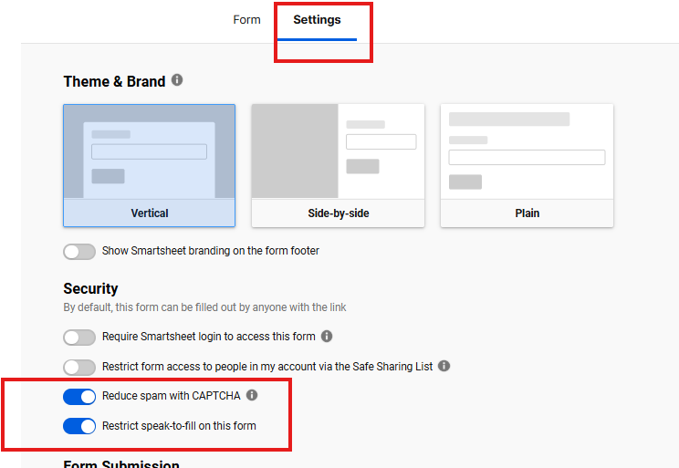
thank you - yes I had done the captcha but not the speak to fill though not sure that will do much either (spam has emojis and links etc) I’d say changing the url is what helped but that’s until it’s picked up again by a bot. I really don’t want to make a new url as our links are in lots of places (like not just on website but in other forms and QR codes made for posters across different sites and tiny urls made of them etc. think 2026 is seeing more powerful AI / spamming bots that’s going to call for more robust defenses
 ChristinaP
Re: Spam from public form
What I did was I enabled the Captcha & Speak-to-Fill. I haven't seen any spam comes through so I hope that fixes it.
The above comment also suggested to make a copy, delete the old form and make a new one. A new URL also help with that.
 Brock
Brock
Spam from public form
We have seen an increase in spam entries from our public forms. I have reCaptcha and "Restrict speak-to-fill" enabled. Hopefully this would help but is there anything else I can do to prevent this?
Brock
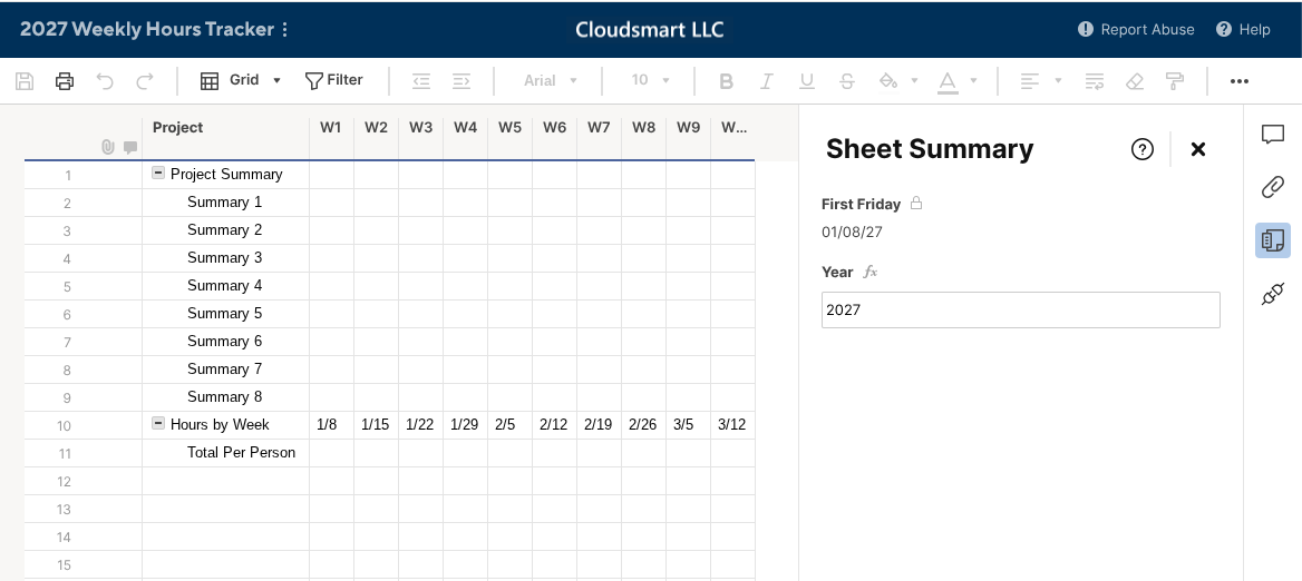
Re: Populate a row with the last Friday of each work week for the year
Hi @sg2034
A not-so-clean solution uses text functions like LEFT, FIND, and MID to get the Day and month values from the '1/9' formatted starting Friday date.
Then, with the day and month values, we create next Friday's date with the DATE function by adding 7 days.
Finally, we use the MONTH and DAY functions to create the display value for next Friday in '1/16' format.
[W1]=MONTH([First Friday]#) + "/" + DAY([First Friday]#)
[W2]=MONTH(DATE(Year#, VALUE(LEFT([W1]@row, FIND("/", [W1]@row) - 1)), VALUE(MID([W1]@row, FIND("/", [W1]@row) + 1, 2))) + 7) + "/" + DAY(DATE(Year#, VALUE(LEFT([W1]@row, FIND("/", [W1]@row) - 1)), VALUE(MID([W1]@row, FIND("/", [W1]@row) + 1, 2))) + 7)
[W3] … Drag and drop the W2's formula.
Then we can drag and drop the W2 formula down to W3 to W52 to populate the cell formulas.
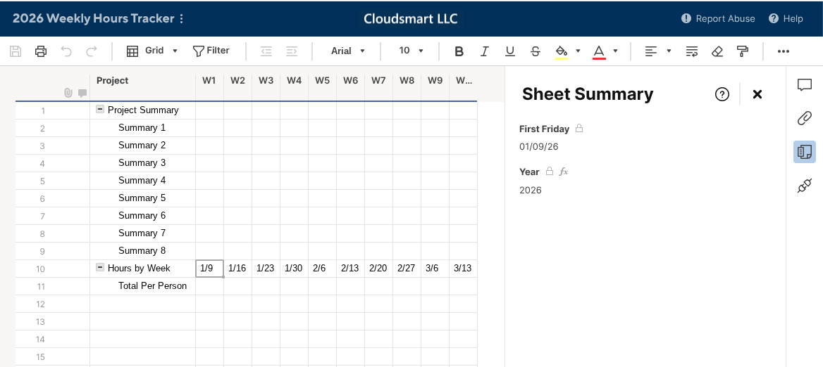
As for the first Friday value, or [W1], and the Year value, I use the Sheet Summary field so that we can copy the sheet and change those values for next year.

Re: Formula help required
@darkmatter I'm most of the way there for my template scenarios (may not work for all edge cases). Do you have a list of project names, or are they going to be new each time?
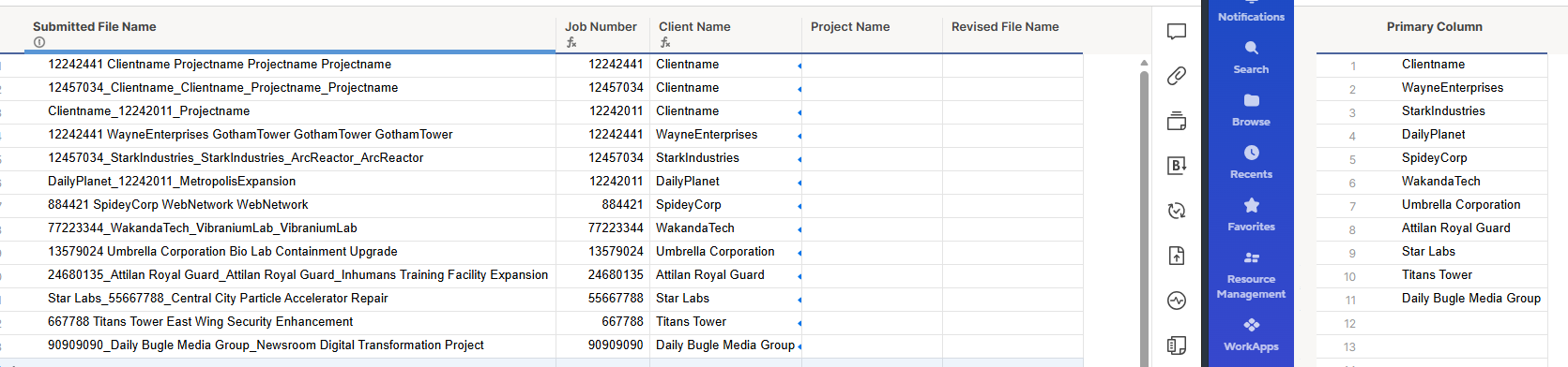
Job Number:
=IFERROR(VALUE(LEFT([Submitted File Name]@row, 8)), IFERROR(VALUE(LEFT([Submitted File Name]@row, 6)), IFERROR(VALUE(MID([Submitted File Name]@row, FIND("_", [Submitted File Name]@row) + 1, 8)), IFERROR(VALUE(MID([Submitted File Name]@row, FIND("_", [Submitted File Name]@row) + 1, 6)), IFERROR(VALUE(MID([Submitted File Name]@row, FIND(" ", [Submitted File Name]@row) + 1, 8)), IFERROR(VALUE(MID([Submitted File Name]@row, FIND(" ", [Submitted File Name]@row) + 1, 6)), ""))))))
Client Name:
=IFERROR(INDEX(COLLECT({Job-Client-Project Client List Range 1}, {Job-Client-Project Client List Range 1}, CONTAINS(@cell, [Submitted File Name]@row)), 1), "")
Once you've got everything separated, you can just concatenate the final list however you want. It'll just come down to whether you can reference a project name list the same way you did the client name or if you need to extract the remaining text once you remove the job number and client name text.
 S.Stone
Re: Meet Sarah Stone, our May Member Spotlight! 🎉
Thanks, Paul! I love that part of WV. I'm originally from up north, about 45min south of Pittsburgh, but we've spent so many years traveling to Blackwater Falls, and my husband and I each rafted the New before we even met. I've got a bit picture of the bridge behind my desk at my home office, too - I may not be standing in Appalachia today, but my heart never left!
I'm excited for the project, too! I've got most of it figured out, but I'm looking to put some polish on it and run it through some testing. Once it's ready to go live, I look forward to hearing your thoughts on it!
S.Stone
Re: Meet Sarah Stone, our May Member Spotlight! 🎉
@S.Stone CONGRATS!
Side note… I am born and raised in WV (and still live there) about 2ish hours away from Blackwater Falls, and we are doing this year's family vacation in the New River Gorge area.
Additional side note… Really looking forward to this new SS idea you're working on. Can't wait to see it!
 Paul Newcome
Re: Best Way to Create a Stacked Bar Chart from multiple columns
Ok. So the multi-grouped reports don't work for building stacked charts as charts can only pull from the first grouping.
This means we will need to create a second sheet and use some formulas with cross sheet references.
In the second sheet you will need the following:
Text/number type column called "Number". This one you are going to manually populate with numbers starting with 1 on row 1, 2 on row 2, so on and so forth. You are going to need to extend these numbers down to accommodate as many leads as you will need, and I suggest a buffer as well. For example, if you know there will never be more than 100 leads, I would extend this column to 150 just to be on the safe side.
The next column will be your Primary Column. I would rename this to "Lead" and use this column formula:
=IFERROR(INDEX(DISTINCT(COLLECT({Source Sheet Lead Column}, {Source Sheet Lead Column}, @cell <> "")), Number@row), "")
Then you are going to have a series of text/number columns that will be one for each phase. They will all have very similar column formulas in them.
=IF(Lead@row <> "", COUNTIFS({Source Sheet Lead Column}, @cell = Lead@row, {Source Sheet Phase Column}, @cell = "Phase 1"))
You would copy/paste this formula into the next phase column, and all you should need to update is the "Phase 1" portion to match whichever phase that column is for.
Next we will create a row report that references this second sheet and is filtered to only show rows where [Lead] is not blank. You are going to want to get rid of the [Sheet Name] column and add in all of the Phase columns.
This row report can then be used to populate your stacked chart.
Paul Newcome