Best Of
Speedometer Chart: Core Product
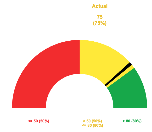
I've noticed a few people asking for Speedometer Charts in Smartsheet, so I figured I would go ahead and publish this solution that I developed. It was some years ago, so there may be better ways and / or more efficient formulas, but this should at least help get everyone started…
A few notes to kick things off…
This solution has been built so that the percentages for each of the three colors is variable.
The indicator width is also variable.
Because we had to get a bit creative, we have to use our own legend and series labels. Since we have to build our own, I figured it wouldn't hurt to get creative with these as well. We can use a section in the underlying sheet with some formulas and conditional formatting to make them more flexible.
Singe the image above is static, I wanted to include that the indicator does move back and forth within the various colored sections to help visualize where within that section you really are.
This allows you to see if you are (for example) towards the lower end of yellow and in danger of going into the red or if you are in the higher end of yellow and almost into the green as opposed to just "yellow".
Basics:
There are three assets in total. A dashboard to display the chart and a sheet to format the data for the chart. These two are the focus of this thread.
The third asset will be your underlying data, but we aren't going to dive into that as there are too many different ways to collect your source data.
Below will be the details as well as screenshots for both the formatting sheet and the dashboard.
Formatting Sheet:
[Primary Column]:
NOTE: All rows in this column are manually entered.
Row 1: "Target"
Row 2: "Actual"
Row 3: "Indicator Width"
[Numbers]:
Row 1: Enter your target number. This number should be equivalent to your "100%" goal.
Row 2: This could be a cell link, a formula with a cross sheet reference, or even manually entered. This is going to be your "Actual" that is represented by the indicator in the chart.
Row 3: This is a manually entered number that indicates how wide you want the indicator in your chart. Lower numbers produce a thinner indicator, and larger numbers produce a thicker indicator. In the snippet above, the indicator width is 1.5.
[Color Label]:
NOTE: All rows in this column are manually entered.
Row 1: "Red" manually entered.
Row 2: "Yellow" manually entered.
Row 3: "Green" manually entered.
[Thresholds (Less Than or Equal To %)]:
NOTE: This column is formatted to show percentages.
Row 1: This will be the maximum percentage that would be considered "Red". For example, if you enter 50%, anything from 0% to 50% will have the indicator somewhere in the red section.
Row 2: This will be the maximum percentage that would be considered "Yellow". Using the example for Row 1, if you enter 80% here, anything above 50% but below 80% will have the indicator somewhere in the yellow section.
Row 3: 100% manually entered.
[Section]:
NOTE: All rows in this column are manually entered.
Row 1: "Red 1"
Row 2: "Indicator 1"
Row 3: "Red 2"
Row 4: "Yellow 1"
Row 5: "Indicator 2"
Row 6: "Yellow 2"
Row 7: "Green 1"
Row 8: "Indicator 3"
Row 9: "Green 2"
[Variable %]:
NOTE: All rows in this column are individual formulas.
Row 1:
=IF(Numbers2 > Numbers@row * [Thresholds (Less Than or Equal To %)]1, 0, (Numbers1 * [Thresholds (Less Than or Equal To %)]1) - ((Numbers1 * [Thresholds (Less Than or Equal To %)]1) - Numbers2) - Numbers3) + 0.00001
Row 2:
=IF(Numbers2 <= Numbers1 * [Thresholds (Less Than or Equal To %)]1, Numbers1 * (Numbers3 / 100), 0) + 0.00001
Row 3:
=IF(Numbers2 > Numbers1 * [Thresholds (Less Than or Equal To %)]1, Numbers1 * [Thresholds (Less Than or Equal To %)]1, (Numbers1 * [Thresholds (Less Than or Equal To %)]1) - Numbers2) + 0.00001
Row 4:
=IF(AND(Numbers2 < Numbers1 * [Thresholds (Less Than or Equal To %)]2, Numbers2 > Numbers1 * [Thresholds (Less Than or Equal To %)]1), (Numbers2 / (Numbers1 * [Thresholds (Less Than or Equal To %)]2)) * (Numbers1 * ([Thresholds (Less Than or Equal To %)]2 - [Thresholds (Less Than or Equal To %)]1)) - Numbers3, 0) + 0.00001
Row 5:
=IF(AND(Numbers2 <= Numbers1 * [Thresholds (Less Than or Equal To %)]2, Numbers2 > Numbers1 * [Thresholds (Less Than or Equal To %)]1), Numbers1 * (Numbers3 / 100), 0) + 0.00001
Row 6:
=IF(AND(Numbers2 < Numbers1 * [Thresholds (Less Than or Equal To %)]2, Numbers2 > Numbers1 * [Thresholds (Less Than or Equal To %)]1), (Numbers1 * ([Thresholds (Less Than or Equal To %)]2 - [Thresholds (Less Than or Equal To %)]1)) - ((Numbers2 / (Numbers1 * [Thresholds (Less Than or Equal To %)]2)) * (Numbers1 * ([Thresholds (Less Than or Equal To %)]2 - [Thresholds (Less Than or Equal To %)]1))), Numbers1 * ([Thresholds (Less Than or Equal To %)]2 - [Thresholds (Less Than or Equal To %)]1)) + 0.00001
Row 7:
=IF(Numbers2 > Numbers1 * [Thresholds (Less Than or Equal To %)]2, MIN((Numbers1 * ([Thresholds (Less Than or Equal To %)]3 - [Thresholds (Less Than or Equal To %)]2)) - (Numbers1 - Numbers2), Numbers1) - Numbers3, 0) + 0.00001
Row 8:
=IF(Numbers2 > Numbers1 * [Thresholds (Less Than or Equal To %)]2, Numbers1 * (Numbers3 / 100), 0) + 0.00001
Row 9:
=IF(Numbers2 >= Numbers1, 0, IF(Numbers2 > Numbers1 * [Thresholds (Less Than or Equal To %)]2, (Numbers1 * ([Thresholds (Less Than or Equal To %)]3 - [Thresholds (Less Than or Equal To %)]2)) - ((Numbers1 * ([Thresholds (Less Than or Equal To %)]3 - [Thresholds (Less Than or Equal To %)]2)) - (Numbers1 - Numbers2)), Numbers1 - (Numbers1 * [Thresholds (Less Than or Equal To %)]2))) + 0.00001
[Legend]:
NOTE: All rows in this column are individual formulas.
Row 1:
="<= " + ROUND((Numbers1 * [Thresholds (Less Than or Equal To %)]@row)) + " (" + ROUND([Thresholds (Less Than or Equal To %)]@row * 100) + "%)"
Row 2:
="> " + ROUND(Numbers1 * [Thresholds (Less Than or Equal To %)]1) + " (" + ROUND([Thresholds (Less Than or Equal To %)]1 * 100) + "%)" + CHAR(10) + "<= " + ROUND((Numbers1 * [Thresholds (Less Than or Equal To %)]2)) + " (" + ROUND([Thresholds (Less Than or Equal To %)]@row * 100) + "%)"
Row 3:
="> " + ROUND((Numbers1 * [Thresholds (Less Than or Equal To %)]2)) + " (" + ROUND([Thresholds (Less Than or Equal To %)]2 * 100) + "%)"
[Metric]:
NOTE: All rows in this column are individual formulas.
Row 1:
=IF(Numbers2 <= Numbers1 * [Thresholds (Less Than or Equal To %)]1, Numbers2 + " (" + ROUND(Numbers2 / Numbers1, 2) * 100 + "%)", 0)
Row 2:
=IF(AND(Numbers2 > Numbers1 * [Thresholds (Less Than or Equal To %)]1, Numbers2 <= Numbers1 * [Thresholds (Less Than or Equal To %)]2), Numbers2 + " (" + ROUND(Numbers2 / Numbers1, 2) * 100 + "%)", 0)
Row 3:
=IF(Numbers2 > Numbers1 * [Thresholds (Less Than or Equal To %)]2, Numbers2 + " (" + ROUND(Numbers2 / Numbers1, 2) * 100 + "%)", 0)
[Actual]:
NOTE: All rows in this column are manually entered.
Row 1, Row 2, and Row 3 all have the word "Actual" anually entered.
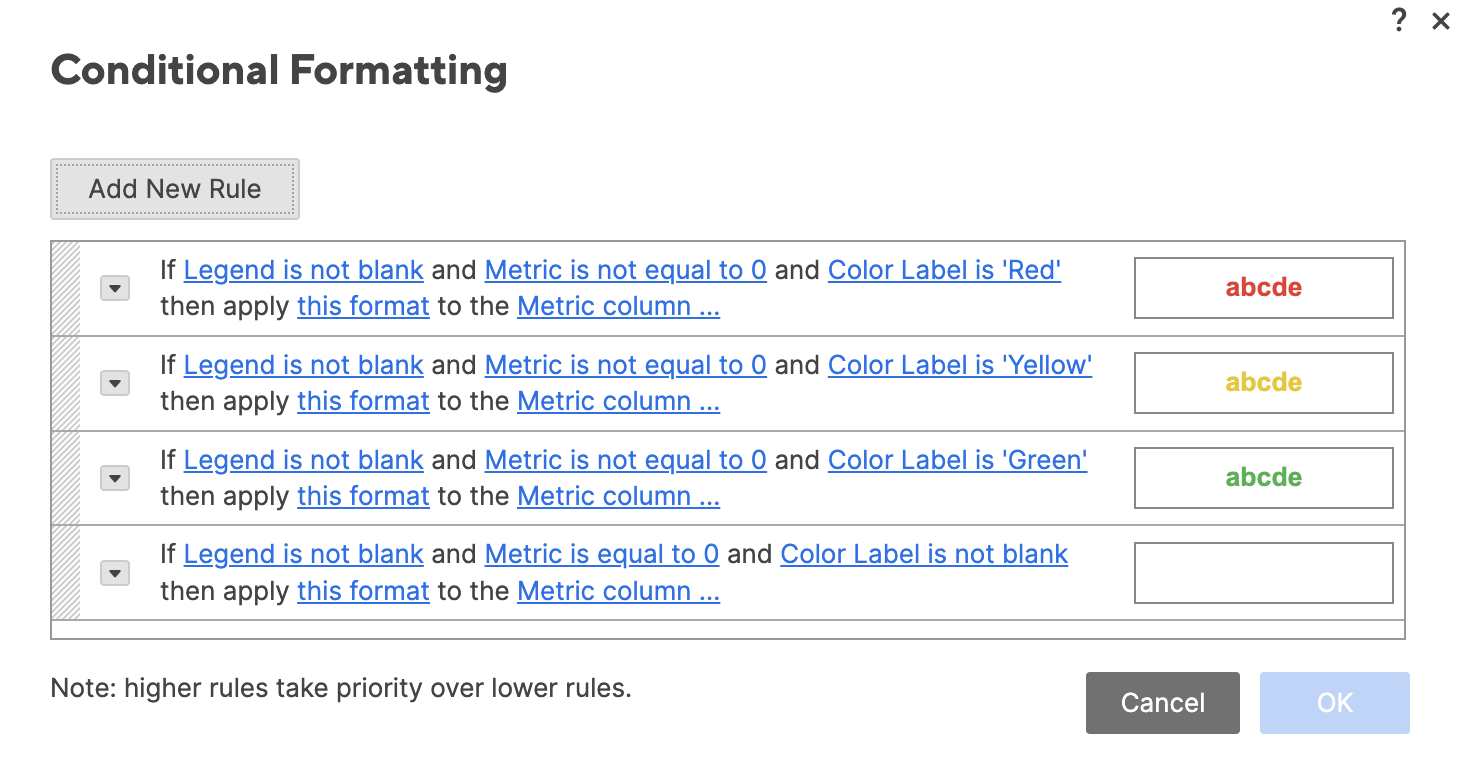
Conditional Formatting:
NOTE: I wasn't able to show it in the screenshot, but each rule is applied to the [Metric] and [Actual] columns.
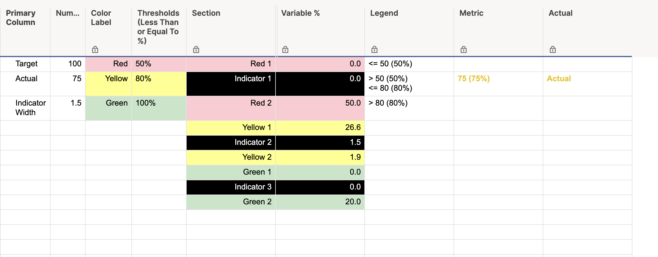
Screenshot of the formatting sheet:
Dashboard:
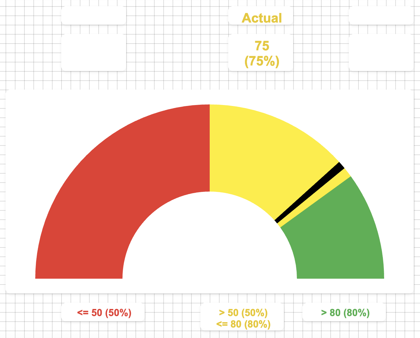
You can use your own judgement for the sizes of each widget, but the general idea here is that we use individual metrics widgets to display the actuals and the "legend", and we use a half-donut chart for the "speedometer" portion.
You can see in the below screenshot how each of the widgets are laid out. I have the "Actuals" going across the top relatively in line with each of their colored sections, and the legend is metrics widgets across the bottom also in line with each of the colored sections.
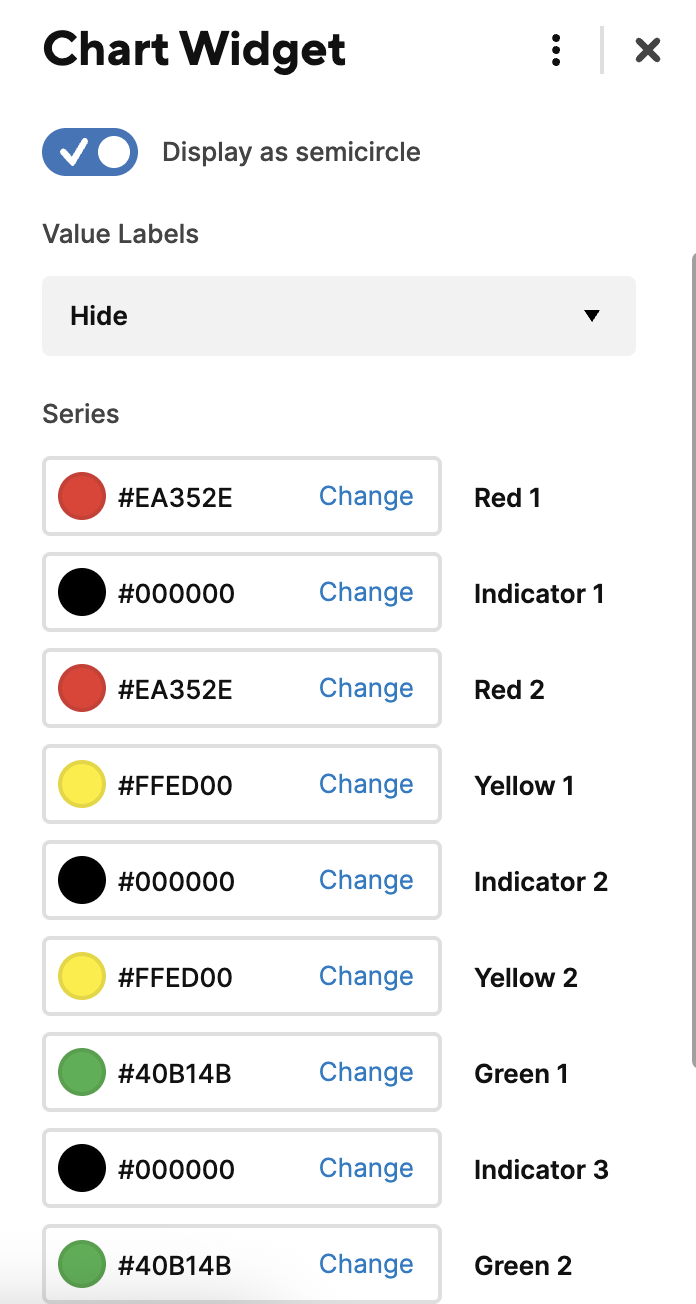
The "star of the show" here though is the speedometer chart. When we select the data for this, we select rows 1 through 9 of both the [Section] column and the [Variable %] column. I will provide a separate snippet of the chart series to show what colors were selected for the above.
Widget Layout:
Series:
 Paul Newcome
Sheet automation notification email tracking using a PowerAutomate Flow and Outlook
This post details how to track all sheet automation notifications emails. This solution is medium complexity and will likely require you to use an AI for some simple coding. Smartsheet allows users to automatically send email notifications from sheets. There are a few significant problems with these automated emails.
- Emails come from automation@app.smartsheet.com and may get junked by the recipient.
- There is no tracking of the emails and users cannot see what emails were sent. This makes auditing impossible.
Users can create an audit trail of automated emails and have them sent from an organization email address using Outlook and PowerAutomate Flows.
What is needed
- Smartsheet sheet automation that sends an email.
- Outlook Shared Email address
- Shared Email addresses are preferred because if staff leaves, the process will still function.
- PowerAutomate Flow
Smartsheet automation configuration
- Setup your automation including the "Alert someone" component.
- Send the Alert to your Outlook Shared Email address.
- Ensure the email subject is unique and easy for a computer to identify.
- PowerAutomate will identify emails for processing based on the subject.
- Ensure the final recipient email is included in the body of the message and a way that is easy for a computer to find. In my example, the final recipient email is always after the string "Instructor email: "
- PowerAutomate will extract the destination email by looking for a string in the email body.
Example automation
Select the Contact column that contains your Outlook Shared Email address. The key areas are highlighted below.
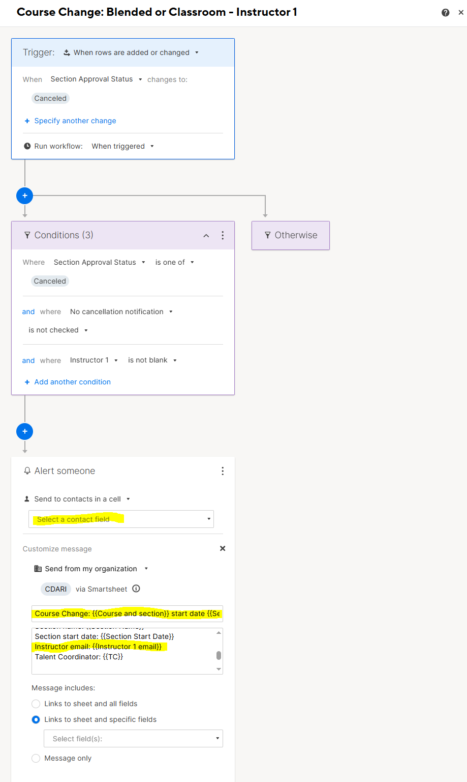
Example email subject
Section Change: {{Course and section}} start date {{Section Start Date}}
Exampled email body
Hello {{Instructor 1 first name}},
I hope you are staying well.
Please note that we have been notified that the section below has been cancelled due to low enrollment. Please accept our apologies for the inconvenience.
Course section: {{Course and section}}
Section name: {{Section Name}}
Section start date: {{Section Start Date}}
Instructor email: {{Instructor 1 email}}
Talent Coordinator: {{TC}}
Kind regards
{{TC}}
Talent Coordinator
Shared Email
This stage will move all the specific automated emails from Smartsheet to an Inbox subfolder for better management and processing by the Power Automate Flow.
- In the SharedEmail Account, create an inbox subfolder for the emails.
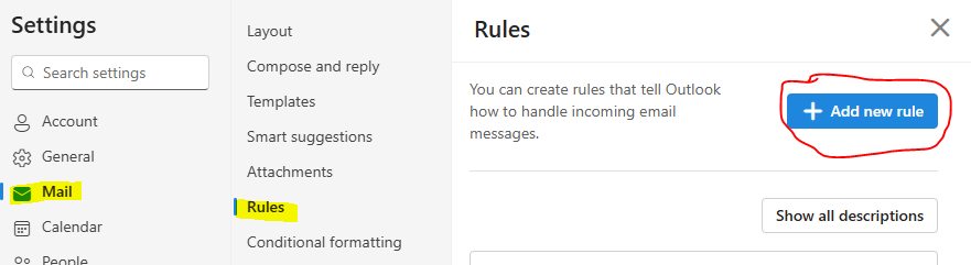
- Create Outlook Rule to put specific emails from automation@app.smartsheet.com in an Inbox subfolder.
- This part of the process requires using Outlook Web and specific navigation.
- Open Outlook Web with your email account that has access to the Shared Email Account
- Click on your icon on the top right and click "Open another mailbox" and type your Shared Email Address.
- This part of the process requires using Outlook Web and specific navigation.
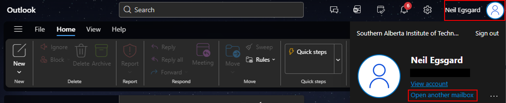
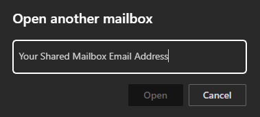
- This will open the shared mailbox where you can edit rules for that mailbox.
- Select Home > Quick Steps

- Select Mail > Rules > Add new rule
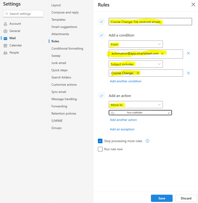
- Setup the rule
- Name
- Add your rule name
- Add a condition
- From
- automation@app.smartsheet.com
- Subject includes
- Your string
- Ex. "Course Change: "
- Stop processing more rules can be checked or unchecked based on your needs.
- From
- Name
PowerAutomate Flow
The PowerAutomate Flow account needs access to view emails and send emails and move emails in the shared email Account. The flow will:
- Check each email for
- From automation@app.smartsheet.com
- Being in a specific inbox subfolder
- Extract the recipient email from the body of the email.
- Send and email from the shared inbox
- Move the sent email to a subfolder of the Sent folder.
Example PowerAutomate Flow
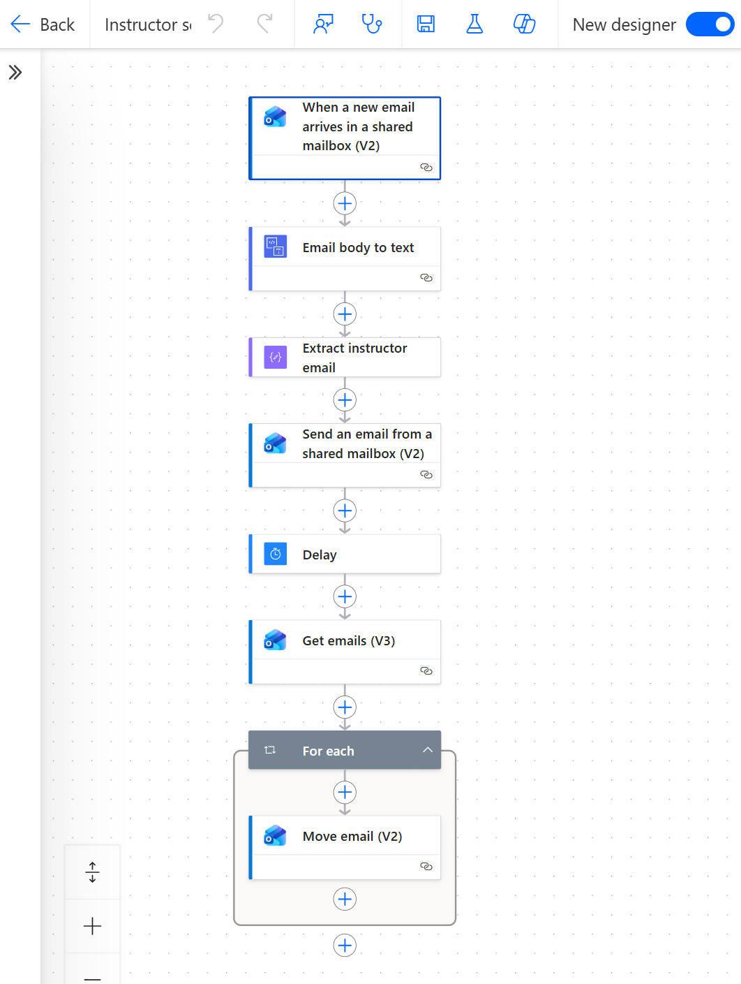
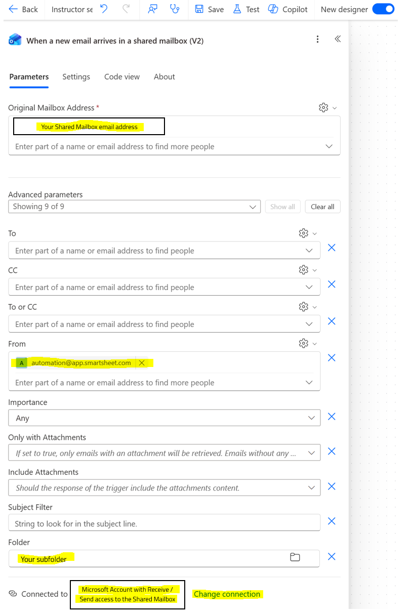
When a new email arrives in a shared mailbox (V2)
Action: Office 365 Outlook > When a new email arrives in a shared mailbox (V2)
This step is the trigger that identifies emails that need to be processed by this flow.
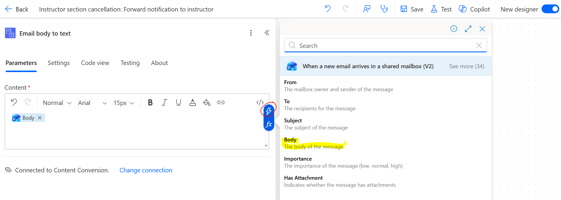
Email body to text
Action: Content Conversion > Html to text
Use the lightning bolt to enter Body variable.
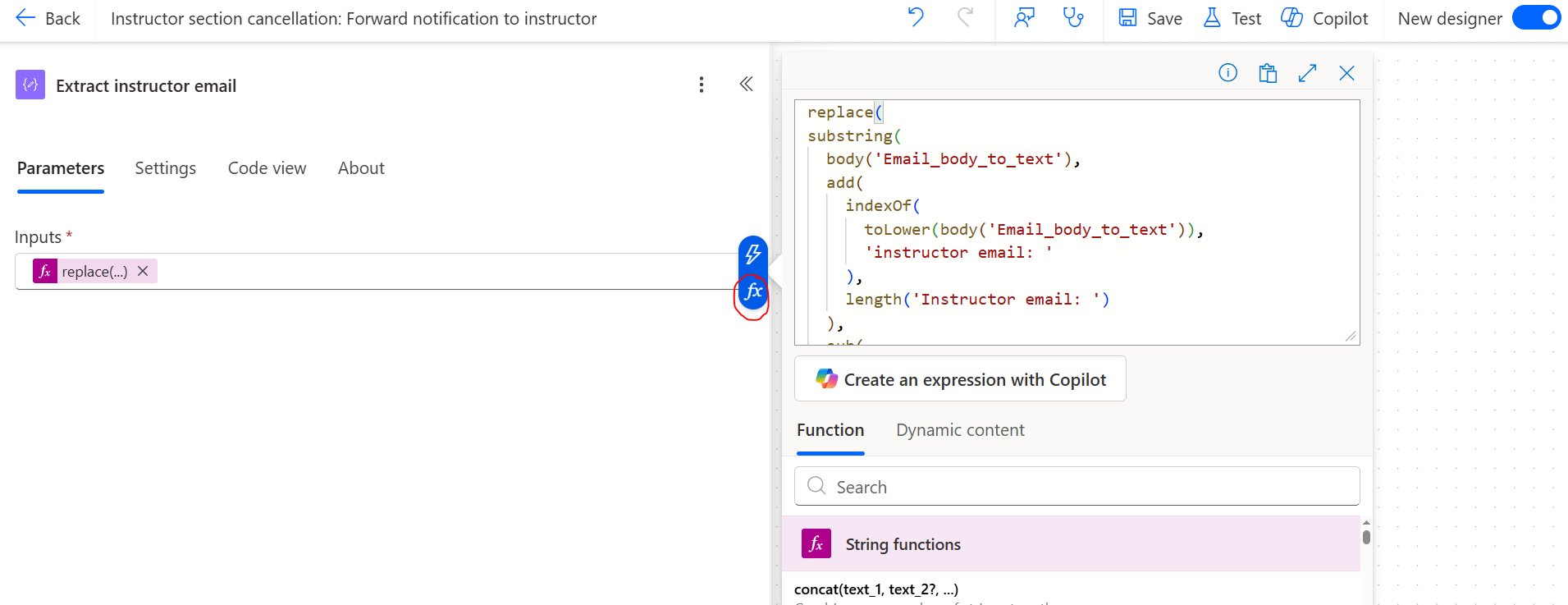
Extract instructor email
Action: Data Operation > Compose
This step extracts the recipient email from the body of the email. In my case I am using the string "Instructor email: " before the email and after "talent coordinator:" so the code can find the email.
Use the Expression button to enter the code. You may need to use an AI to adjust the code to your needs.
Code
replace(

substring(

  body('Email_body_to_text'),

  add(

    indexOf(

      toLower(body('Email_body_to_text')),

      'instructor email: '

    ),

    length('Instructor email: ')

  ),

  sub(

    indexOf(

      toLower(body('Email_body_to_text')),

      'talent coordinator:'

    ),

    add(

      indexOf(

        toLower(body('Email_body_to_text')),

               'instructor email: '

      ),

      length('Instructor email: ')

    )

  )

)

,decodeUriComponent('%0A'),'')
Send an email from a shared mailbox (V2)
Action: Office 365 Outlook > Send an email from a shared mailbox (V2)
This step will send the email.
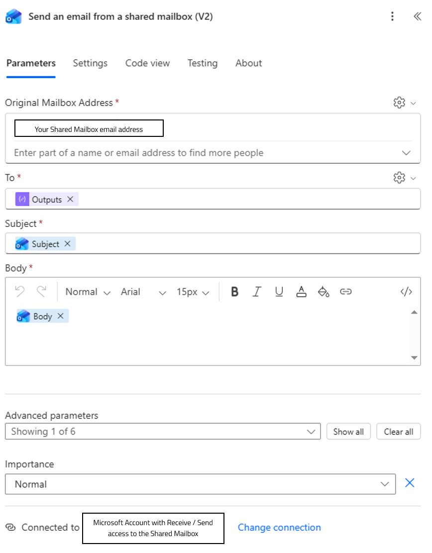
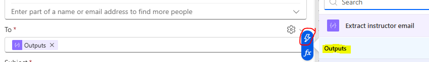
Below are screenshots showing to use the lightning bolt to get the correct variables.
To
Subject
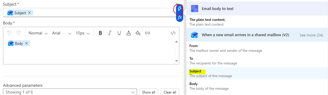
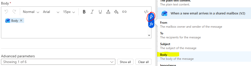
Body
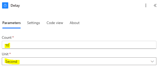
Delay
Action: Schedule > Delay
This step allows the email to finish sending before trying to move the sent email to a storage folder. If the delay is not used, the sent email is not moved because it does not exist.
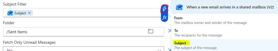
Get emails (V3)
Action: Office 365 Outlook < Get emails (V3)
This step finds the email that was just sent by:
- Matching the subject
- looking in the Sent folder
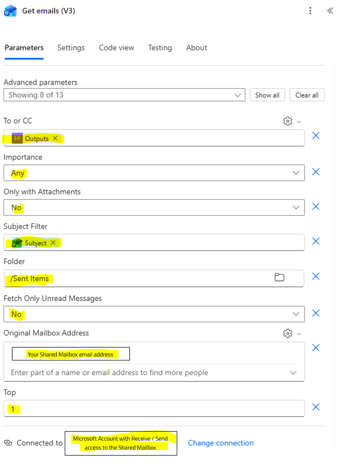
Below are screenshots showing to use the lightning bolt to get the correct variables.
To or CC
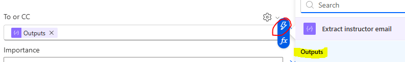
Subject Filter
For each
Action: None. This will be automatically added then you add the "Move Email (V2)" action.
This step runs the "Move Email (V2)" for every email found in the Get emails (V3) step.
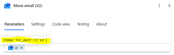
Move Email (V2)
Action: Office 365 Outlook > Move Email (V2)
This step moves the sent email to a subfolder for better organizing and ease for auditting.
Add this action will automatically create the "For each" loop.
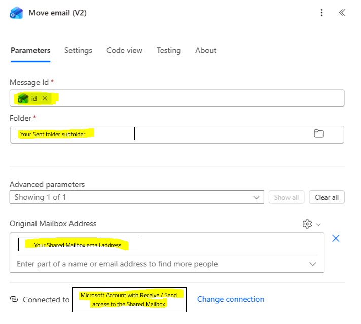
Below are screenshots showing to use the lightning bolt to get the correct variables.
Message Id
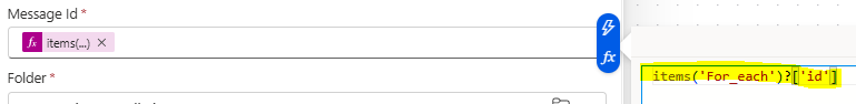
When you save and refresh the flow, the Message Id icon will change to the below.
Summary of results
This setup allows you to have Smartsheet notification emails that are:
- Sent from your business email
- Provide an audit trail of automated email history
Have a good day and I hope this is useful.
Neil Egsgard
Business Solutions Architect
Southern Alberta Institute of Technology
 Neil Egsgard
Re: A memorable year for the Smartsheet Community
What an exceptional write-up to celebrate the amazing achievements on ‘25 - Congratulations!
Amazing statistics for an amazing community!
 Protonsponge
Controlling record visibility in reports using Smartsheet Groups
This solution allows you to combine the "Current User" filter and Smartsheet Group membership to filter records based on who is a member of a Smartsheet Group.
Solution overview
- Python
- Create scheduled task to run daily Python script that pulls all Smartsheet groups and group members and saves as CSV on SharePoint site.
- DataShuttle
- Schedule DataShuttle to load "Group-Member" CSV into "Groups" DataTable
- DataTable
- Create DataTable Connection to load "Groups" DataTable data into "Group-Members" sheet.
- Group-Members sheet
- The "Group-Members" sheet will contain a record for each Group-Member combination. There will be one record for every member of every group.
- DataMesh - Group names to Group Summary sheet
- Create DataMesh to transfer Group names from "Group-Members" sheet to "Group Summary" sheet.
- Group Summary sheet
- The "Group Summary" sheet will contain a list of every group and all members. There will be one record per Group.
- On "Group Summary" sheet use a Join Collect formula to gather all the group member emails into the "Group members - Text" field.
- =IF([# of members]@row <= 30, JOIN(COLLECT({Smartsheet Group List - Member email}, {Smartsheet Group List - Group name}, [Smartsheet group name]@row ), ";"), "Too many members to display")
- The Group members will appear as emails separated by ";"
- DataMesh - Convert member emails into Contacts
- Create a DataMesh to transfer the text group members into a Contact column called "Group members" on the same "Group summary" sheet. The text emails will be converted into Contacts.
At this point you will now have a automatically updating list of groups with their members as Contacts in Smartsheet. You can you DataMesh or cros ssheet references to pull the Group members onto other sheets using the Group name.
Tools required
- Computer to run scheduled Python query to pull Groups and Group members and save it to a SharePoint location
- SharePoint location to save the Group-Member list
- Smartsheet API access
- DataShuttle
- DataTable
- DataMesh
I hope this is useful to you.
Neil Egsgard
Business Solutions Architect
Southern Alberta Institute of Technology
Neil Egsgard
Formula to add Months to Date
This is the simplest formula I can find to add Months to Date. This considers sum of months exceeding 12, converting it to January and adding 1 to the year.
Where: Term column is the number of months to add, Date is the starting date.
=DATE(
  YEAR([Date]@row) + INT((MONTH([Date]@row) + [Term]@row - 1) / 12),
  MOD(MONTH([Date]@row) + [Term]@row - 1, 12) + 1,
  DAY([Date]@row)
)
Posting it out here for my future use. I surely will forget this when I need it.
 heyjay
The new Overachievers are here! 🤩

Community, join me in congratulating our 13 incoming and incredible Smartsheet Overachievers who will be joining our returning members this year!
- @AdamSYNH (Adam Collins)
- @A.Veloso (Andrei Veloso)
- @florian.zbinden7
- @Isis Taylor
- @Ide AirTrunk (Jamie Ide)
- @joey.w.razzano
- @kmalone51256 (Karen Malone)
- @Karen_Pytel
- @Kristen Christman
- @Protonsponge (Louis Leir)
- @Monique Odom Stearn
- @Scott Gehrig
- @Sing C
⭐️ Meet the entire collective here ⭐️
These Smartsheet customers have a passion for achieving the impossible - and most importantly, helping others do the same. They represent different industries, roles, global regions, Smartsheet superpowers, and more. Alone, they are amazing, but together? That's when the magic happens.
Not only will they be representing customer feedback and relaying to our greater team, but they'll be here for you, too. You'll be seeing them at ENGAGE this year and beyond as they tell their stories, share their knowledge, and help others in community.
We've also just launched a new page that shows all Overachiever Alumni and will help you get to know them as well! Check them out, including the Founding Members class from 2020.
The next application season will open at the beginning of Summer 2026 - make sure you're notified by signing up here. Until then, join me in celebrating these folks today and for the next few weeks, including on social. A special shoutout to our Community Champions who were selected - we love watching your growth!
So much more to come! (You know I had to end on a classic jam 🎵)
 Alison C.
Power Automate - Post Attachments to Row/Sheet
Hello everyone!
I spent WAY to long looking for this answer so I thought I would share it with the Community in hopes of helping someone else.
Problem: Adding attachments to rows/sheet is not possible through the standard SmartSheet Connector
Solution: This can only be done by creating a Custom Connector. It CANNOT be done through the HTTP request. As of writing this, here is the relevant information. On the
General tab
Scheme: "HTTPS"
Host: "api.smartsheet.com"
Base: "/2.0/"
Security
Authentication Method: API Key
Parameter Location: Header
The rest of the info is up to you.
Definition
Url: https://api.smartsheet.com/2.0/sheets/{sheetId}
Headers: Content-Type and Content-Disposition
Body: This must be edited in the swagger editor after creating Action. The body should look like this
" - name: file
in: body
required: false
schema:
type: string
format: binary
"
Be sure to format it consistent with the rest of the Yaml.
The rest of the info is up to you.
Finally Update the connector. You should now be able to use this custom connector in your flows.
Your Atachtion should look like the example below. Key items, you will need to know the Content-type. If you are using ShareFile, you can get it directly from the "Get File Content" step. Just be sure to drill down from the body, ie. @{body('Get_file_content')?['$content-type']}. I used the Get File Metadata step to get the file name. You will need the file extension but not the folder path. Finally, the File MUST be in Binary. If your file is in Base64, use the following: @{base64ToBinary(body('Get_file_content')?['$content'])}
I hope this helps!
 jordanfritz513
[CLOSED] Dungeons & Dragons Team is seeking for Smartsheet Expert Producer!
6 months Contractor position
All the details are in the link. If you have additional question, please contact them directly.
https://careers.hasbro.com/careers/job/68750265810
Thanks!
 Chizu Hieida
Re: Freeze Rows
Hi @Eric Harwood,
I recommend up voting this feature request! This will help the Smartsheet team prioritize this feature faster, and other people will be more likely to see the big feature request.
Best!
 SSFeatures
Re: How can I get the column to accurately track hours elapsed?
@GasserE Does this video help?
 Darren Mullen