Best Of
Extend "Request an approval" workflows to more than 2 options
Approval workflows allow you to approve or deny something, and the result is tracked by choosing a particular state from a dropdown menu.
There could be many more than 2 desired state outcomes from a review request, for example:
- Pushback: I will not deny this yet, but it needs work before I will approve
- Approved with caveats
- Any other outcome that generates an action based on the chosen state from the dropdown menu
Basically, I'm asking for more buttons than just "Approve" & "Deny" to be able to follow multiple pathways following the review.
 Bruce Northcote
SORT with Automation
Why can we not SORT a worksheet through automations???
This seems SO basic. When we add data to a worksheet, or move data out of a worksheet, it makes sense that we would need to Re-Sort that worksheet, but we still can't do so through automation.
I have about a dozen worksheets where I am adding, moving, or changing data overnight through automations and every morning I spend 30 minutes resorting those worksheets because I have added new data or changed existing data.
DELETING lines would also be nice, but I somewhat understand why we don't have that option, and there are simple work arounds (like moving data to an archive sheet). But there is NO work around for sorting new or changed data.
 Paul Perger
Re: Urgent: My Form Is Spamming Users with Bitcoin Links and I Cannot Deactivate It
In addition to Paul's note, I would also recommend reporting any instance of spam to Smartsheet by using the Abuse form here:
Thank you!
Genevieve
 Genevieve P.
Re: SmartStories - Beschreiben Sie Smartsheet für die Neulinge!
Vielen Dank!
Ja stimmt:
Single Source of Truth
Transparency
Simplicity
Smartsheet
 Mickael Osswald
Get Existing Report Definition via API
I have plenty of use cases where being able to get a report's existing definition would be really useful. We can update it via API, but we currently can't retrieve it.
 Paul Newcome
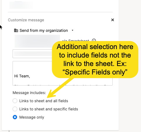
Ability to Include selected fields in Smartsheet Notifications - With out the Link to SMARTSHEET.
It would be great to have the ability to exclude link to the smartsheet while including smartsheet fields in smartsheet automated notifications. This is because we want users to use dynamic view instead of directly accessing smartsheet. With dyamic view we can control what they see and what they can edit.
 ligeshgopi
Re: Duplicating a Large Workspace
@Paul Newcome I'm running into this issue as well. I'm building a PMO workspace that's already over the 100-sheet limit (that's with only 50% of the workspace created so far). There are a LOT of cell linking/copy row functions that would be crazy to have to redo every time a new project folder is created.
Have any workarounds been created for this? Or has anyone heard if Smartsheet plans to up the limit? (around 250 sheets would be nice...) 😁
ShelbyWarren
Re: Linked contact list support - now generally available!
When will multi-select be supported?
 Andrée Starå
Feature request: Portfolio roadmap view
Summary
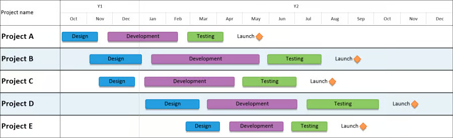
Introduce a new roadmap visualisation within Smartsheet that allows multiple tasks or phases belonging to the same project to be displayed on a single row. This would provide a true portfolio-level roadmap view similar to those available in dedicated roadmap products, whilst retaining Smartsheet as the system of record.
Current challenge
Smartsheet's existing Gantt and Timeline views are task-centric. Whilst excellent for project execution and detailed planning, they are less effective for portfolio-level communication where stakeholders need to understand how projects progress through key phases over time.
Today, projects are commonly structured as:
- Project A
- Design
- Development
- Testing
- Launch
In Gantt View, each phase appears on a separate row. In Timeline View, tasks are also displayed independently. This makes it difficult to create executive-level roadmaps where projects occupy a single visual lane and multiple phases are displayed sequentially across a timeline.
As a result, many customers export Smartsheet data into Power BI or similar tools purely to create roadmap visualisations.
Proposed Solution
Introduce a new Roadmap View that:
- Displays one row per project.
- Allows multiple date ranges to be rendered on the same row.
- Supports colour-coded project phases.
- Supports milestone markers.
- Supports grouping and filtering.
- Supports programme and portfolio roll-ups.
- Maintains a live link to underlying task data.
Key Capabilities
Multi-Bar Rows
Allow multiple bars to be displayed on a single project row, each mapped to different date fields.
Milestone Support
Display milestone icons alongside phase bars.
Dynamic Phase Mapping
Allow users to select:
- Start date column
- End date column
- Colour
- Label
for each roadmap phase.
Portfolio Filtering
Support filtering by:
- Client
- Programme
- Project Manager
- Region
- Status
- Custom fields
Dashboard Integration
Allow Roadmap Views to be embedded directly within Smartsheet Dashboards.
Hierarchy Grouping
Allow projects to be grouped under programmes, portfolios or business units whilst maintaining a concise roadmap view.
Why This Is a Strong Candidate for Enhancement
Timeline View already contains much of the underlying functionality required.
The enhancement is not the creation of an entirely new module, but rather the ability to render multiple date ranges against a single record or row.
From a user perspective, this feels like a natural evolution of Timeline View rather than a completely new product area. The underlying project data already exists within Smartsheet; customers simply need an alternative visualisation optimised for portfolio reporting.
Business Value
Executive Reporting
Provides an executive-friendly portfolio roadmap without requiring external tools.
Reduced Tool Sprawl
Many customers currently export Smartsheet data into Power BI or roadmap-specific products purely for visualisation. This feature would eliminate a common reason for leaving the platform.
Increased Stakeholder Adoption
Executives, PMOs and clients typically want roadmap views rather than detailed task schedules. Providing both within Smartsheet would improve adoption across a wider audience.
Improved Dashboards
Roadmaps are one of the most common artefacts presented in steering groups, governance forums and client reviews. Native support would significantly strengthen Smartsheet Dashboard use.
Competitive Positioning
Brings Smartsheet closer to roadmap capabilities offered by competitors e.g.
- Monday.com Portfolio Views
- Microsoft Project Roadmap
whilst retaining Smartsheet's flexibility and work management strengths.
Example Use Cases
- Programme roadmaps
- Product launch planning
- Construction project portfolios
- PMO reporting
- Agency campaign planning
- Transformation programme governance
- Client-facing delivery roadmaps
Success Criteria
- Projects displayed as a single lane with multiple phases.
- Multiple date ranges displayed on the same row.
- Milestone support.
- Dashboard embeddable.
- Fully filterable and reportable.
- No requirement for duplicate project data.
- Live connection to underlying schedules and task updates.
 darkmatter
Re: Spam from public form
We are having the same issues. We are a not for profit club with numerous public facing form links on our club website and numerous documents etc. Captcha does not seem to change anything. I am unsure what the Restrict to Speak option is so will try this, but it sounds like it may not make much difference.
Lbanangu