What is the best formula to pull in the contents in a cell in the same column even if the original row is deleted?
Background: I'm building a Profile Data sheet for a new blueprint. This blueprint has several optional project plans. Each plan will be on the profile data, capturing things like Start/End dates, schedule variance, overdue and blocked tasks. I need those stats to roll up to the Portfolio summary, so I need the Summary section to pull the stats from the specific project plan metrics starting on row 69. Once the project is provisioned, the other project plans' profile data will be deleted from the Profile Data sheet which means the project plan metrics will always start on row 69.
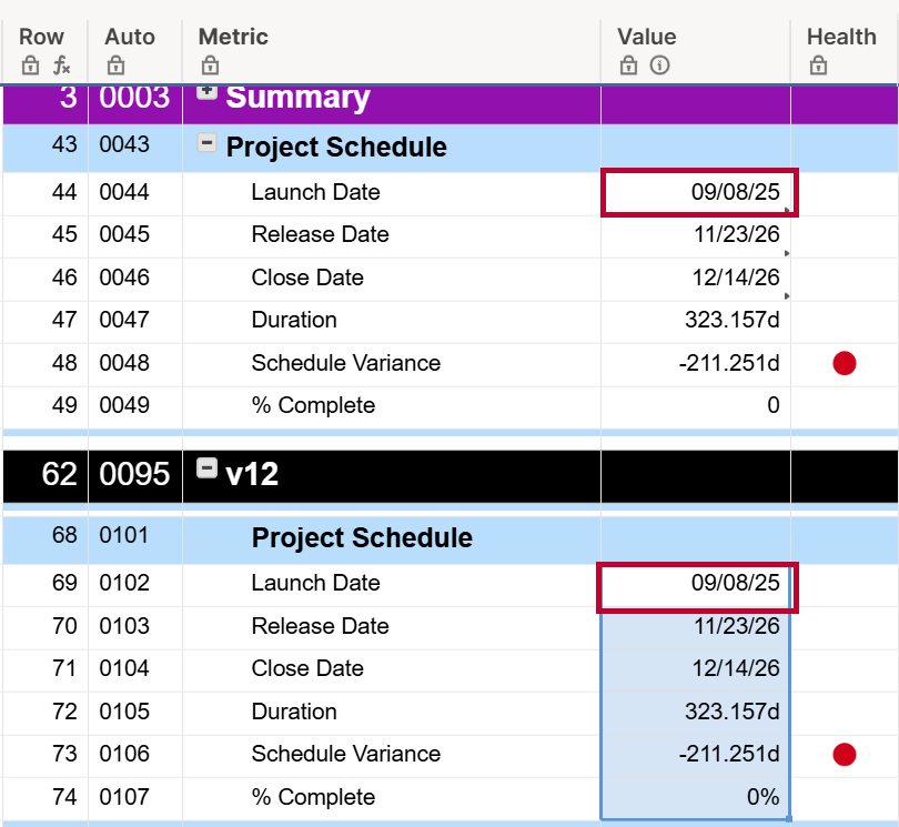
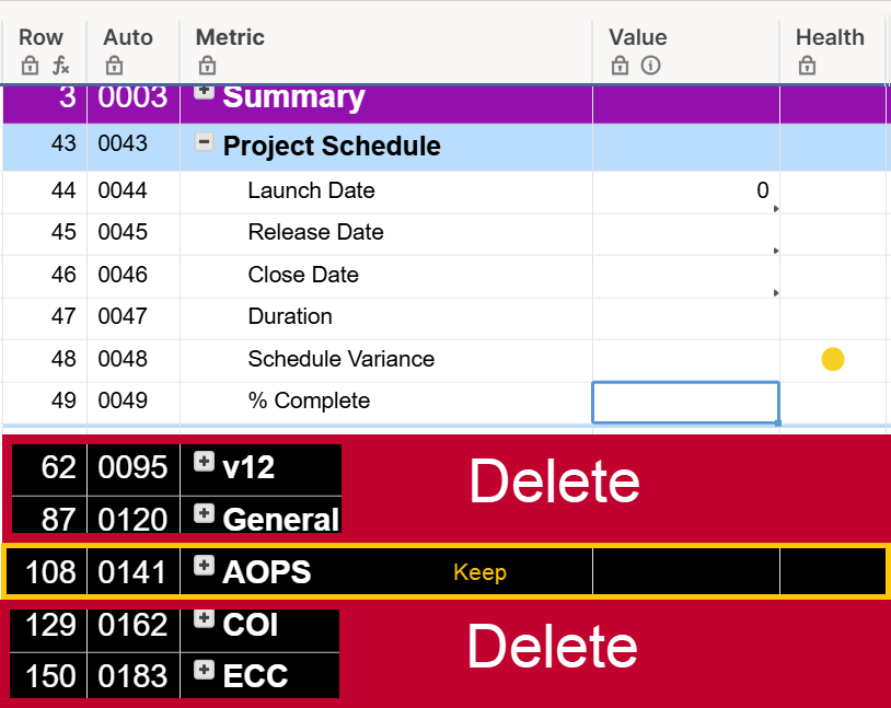
For example, my project will be AOPS. The v12, General, COI, and ECC project sections will be deleted, therefore AOPS Launch Date will be on row 69. I need Value44 to always pull Value69 even if the original row 69 is deleted.
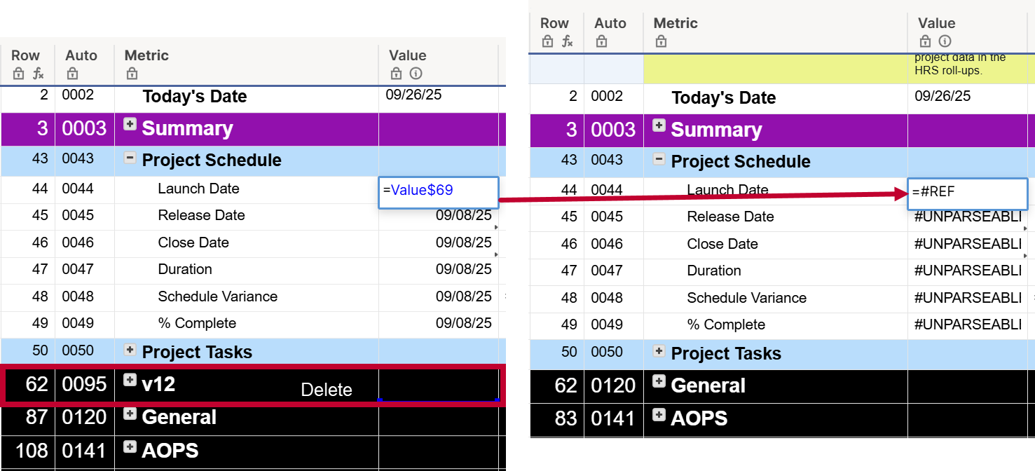
If I use =Value$69 in Value44, it gives #Unparseable when I delete v12 project plan.
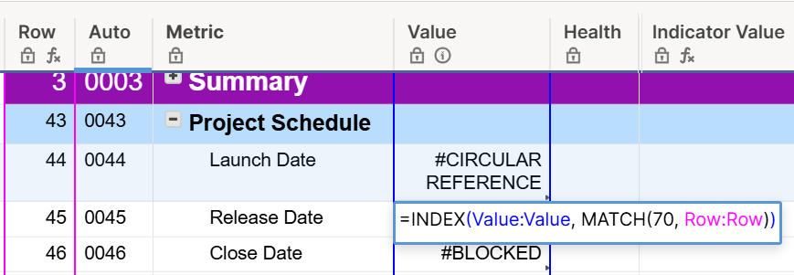
If I use =INDEX(Value:Value, MATCH(69, Row:Row)) in Value44, it pulls the launch date, but as soon as I put =INDEX(Value:Value, MATCH(70, Row:Row)) in Value45, I get a #CircularReference in Value44 and #Blocked in Value 45. Same thing if I use Index/Match in a helper column instead of the same Value column.
If it matters, the contents in the Value69-74 will be linked in from the corresponding project plan, but it just has text values for now, yet it is still throwing errors.
Is it possible to achieve this objective? If so, what is the best formula to do that? I welcome suggestions for alternative ways to capture project plan metrics regardless of the plan that is selected.
