(RANKEQ) Derivative Numbering System e.g. 1a, 1b, 2a, 2b, 2c etc.

Jim B

Hello, I’m a bit stuck with creating a numbering system – can anyone help please?

I have a list of IDs, but some of these IDs I want to mark as derivatives of others and automatically label the derivatives with a letter ideally – but a number will do.

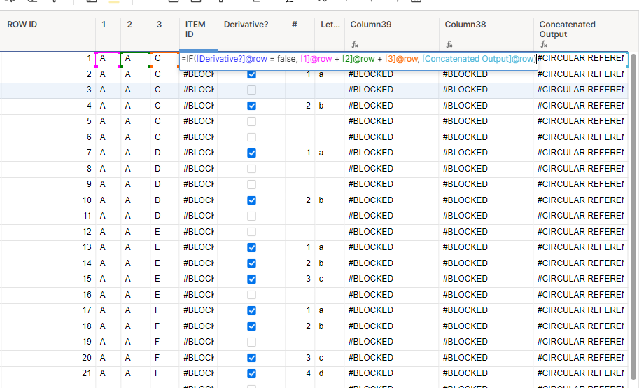
I need my formula to look down a column, count distinct numbers and where [Derivative?] is True assign a rank within that range of distinct numbers.

So the first item in that ‘group’ of distinct numbers that is checked True will be 1 (or a), the second in that group would be 2 (or b) and so on. From there I can relate the number to a letter and concatenate the results to give me my output Item ID.

I have another row ID column that is autonumbered that could drive the ranking.

Or am I overthinking this?

Hope someone can help.

Many thanks,

Jim

Katie G

@Jim give this a try:

=[Item ID]@row + IFERROR(CHAR(96 + RANKEQ([Row ID]@row, COLLECT([Row ID]:[Row ID], [Item ID]:[Item ID], [Item ID]@row, [derivative?]:[derivative?], 1), 1)), "")

Katie G

The COLLECT function is one of my absolute favorites! In this formula, first it finds the set of row ID #s that have the same Item ID, are checked off as derivative, to know which one to rank.

Then I'm taking advantage of the CHAR function https://help.smartsheet.com/function/char and the fact that the character number for a lower case "a" is 97. So if rank = 1, it does 96+1 to know that it's an "a". This will fail if you have more than 26 derivatives, so you might need to modify in that case.

Katie G

Not sure if I'm following correctly, but I think maybe a solution is moving that logic into the formula to prevent the circle?

=[1]@row + [2]@row + [3]@row + IFERROR(CHAR(96 + RANKEQ([Row ID]@row, COLLECT([Row ID]:[Row ID], [1]:[1], [1]@row, [2]:[2], [2]@row, [3]:[3], [3]@row, [derivative?]:[derivative?], 1), 1)), "")

Or another might be having an intermediate "helper" column then the ultimate output of ITEM ID.

Katie G

@Jim give this a try:

=[Item ID]@row + IFERROR(CHAR(96 + RANKEQ([Row ID]@row, COLLECT([Row ID]:[Row ID], [Item ID]:[Item ID], [Item ID]@row, [derivative?]:[derivative?], 1), 1)), "")

Jim B

Perfect, Katie. Thank you so much.

Now to figure out how you did it!

All the best,

Jim

Katie G

The COLLECT function is one of my absolute favorites! In this formula, first it finds the set of row ID #s that have the same Item ID, are checked off as derivative, to know which one to rank.

Then I'm taking advantage of the CHAR function https://help.smartsheet.com/function/char and the fact that the character number for a lower case "a" is 97. So if rank = 1, it does 96+1 to know that it's an "a". This will fail if you have more than 26 derivatives, so you might need to modify in that case.

Jim B

That is so brilliant. Thank you, Katie. Jim

Jim B

I fixed it. Phew.

sorry @Katie G, me again. I ran into a problem here with a circular reference.

Didn't see this coming so I did not think to mention that the [Item ID] is a concatenation of 3 other columns and if [Derivative?] is checked I want to used the [Concatenated Output] rather than [1]+[2]+[3].

This means the IF formula in the [Item ID] column cannot run because it is referring to itself.

Is there a workaround here?

Thanks,

Jim

Katie G

Not sure if I'm following correctly, but I think maybe a solution is moving that logic into the formula to prevent the circle?

=[1]@row + [2]@row + [3]@row + IFERROR(CHAR(96 + RANKEQ([Row ID]@row, COLLECT([Row ID]:[Row ID], [1]:[1], [1]@row, [2]:[2], [2]@row, [3]:[3], [3]@row, [derivative?]:[derivative?], 1), 1)), "")

Or another might be having an intermediate "helper" column then the ultimate output of ITEM ID.

Jim B

Thank you for your help, Katie.

Jim