INDEX-MATCH formula using cross-sheet references

Hi,

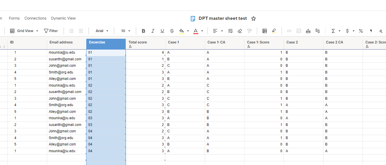
I am collecting data for the surveys, and this survey was asked to complete once per month throughout the year. The sheet has columns like, Email address, Name, Institution, Country, Exercise No (01,02,03,04,05,06 etc.) Case 1, Case 2, case 3, Case 4 (dropdowns). The participants complete the survey every month, and I've figured out to delete the duplicates and the ways to give score (1/0) by including additional columns.

Source sheet:

Now, I have created another sheet, to track the number of exercises each participant has completed, by copying all the email addresses and also to track the ongoing total for each participant. This sheet has Email address (manually fed, for now), Total no. of exercises completed (Finding ways to automate this column, based on email address and referencing it back to source sheet with email and exercise), total score for exercise 1, total score for exercise 2, total score for exercise 3, total score for exercise 4, (etc. until 12), and Overall score. This way, each participant information will be contained in a single row.

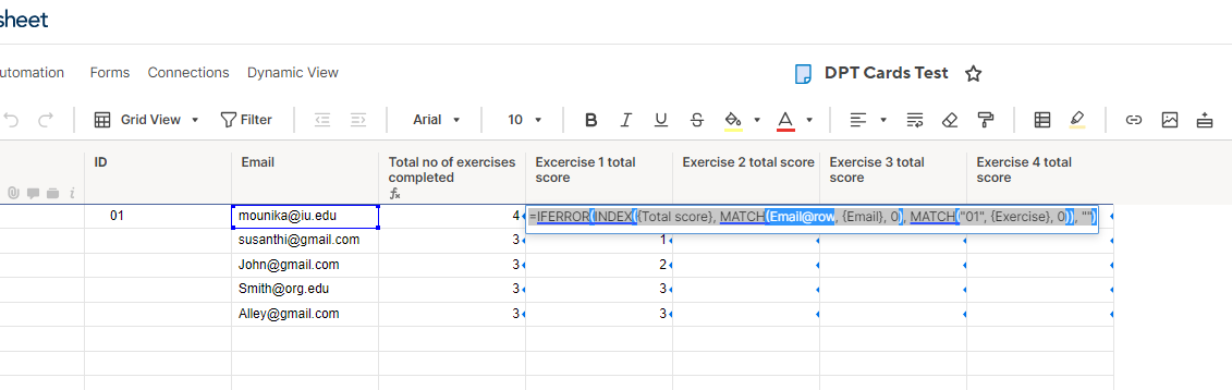
Destination sheet:

Within this destination sheet, I have created a cross sheet references Email, Total score, and Exercise.

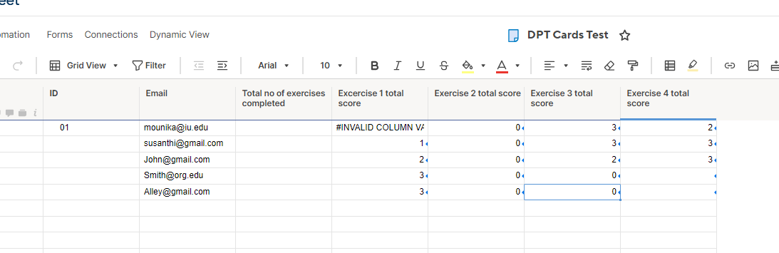
For Excercise 1 total score: =IFERROR(INDEX({Total score}, MATCH(Email@row, {Email}, 0), MATCH("01", {Exercise}, 0)), "") , thus formula worked as expected, it pulling the right total score for each email address.

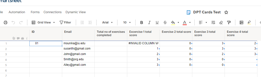
For Exercise 2 total score: =IFERROR(INDEX({Total score}, MATCH(1, (Email@row = {Email}) * ("02" = {Exercise}), 0)), 0), however, I have tried using the same above formula (used for Exercise 1 total score) but didn't worked, and tried this formula which is generating 0 for all.

Can someone please help me identify what is going wrong?

And also any suggestions on how to populate the column "Total no of excercises completed" (this would be the number of times the email address was present in the source sheet".

Thanks in advance!

Find more posts tagged with

Accepted answers

All comments

Aman Shah

The error in your formula for Exercise 2 is due to incorrect syntax for the MATCH function. Here's a corrected version of the formula:

=IFERROR(INDEX({Total score}, MATCH(Email@row, {Email}, 0), MATCH("02", {Exercise}, 0)), "")

Ensure that the {Total score}, {Email}, and {Exercise} references are correctly set up as cross-sheet references. 


This formula should correctly pull the total score for Exercise 2 based on the email address.

For the "Total number of exercises completed" column, you can use the COUNTIF function:

=COUNTIF({Email}, Email@row)

I would also recommend using a combination of the INDEX-COLLECT function as follows:



=IFERROR(INDEX(COLLECT({Total score}, {Email}, Email@row, {Exercise}, "02"), 1), "")

Hope this helps :)

Regards,

Aman Shah

Partner Enablement Manager, Asia Pacific and Japan

Mounika

@Aman Shah

Thank you so much for the response. Apologies, I've just realized that I provided wrong screenshot for the source sheet. Here is the right one.

Source sheet:

The exercise column is single column, which has different values.

Destination sheet:

I have applied and tried both the formulas you have suggested, and they are returning 0 🥲.

Exercise 1 total score : =IFERROR(INDEX({Total score}, MATCH(Email@row, {Email}, 0), MATCH("01", {Exercise}, 0)), "") (this is working as needed)

Exercise 2 total score : =IFERROR(INDEX({Total score}, MATCH(Email@row, {Email}, 0), MATCH("02", {Exercise}, 0)), "")

Exercise 3 total score : =IFERROR(INDEX({Total score}, MATCH(Email@row, {Email}, 0), MATCH("03", {Exercise}, 0)), "")

Exercise 4 total score : =IFERROR(INDEX({Total score}, MATCH(Email@row, {Email}, 0), MATCH("04", {Exercise}, 0)), "")

I have re-checked all the cross-sheet references and all are referenced correctly (if not, the formula for "Exercise 1 total score" also should not work, which is working in my case).

I would also like the formula to return (numeric) 0 if no email is matched for that specific exercise.

Please help me! And the formula for "Total no of exercises completed" was working as needed. Thank you so much again! Looking forward to hear back from you!

Sign in to join the conversation!

Quick Links

Component react.discussion.discussions had an error.

ref must be one of: categoryID, siteSectionID, category, category/categoryID, category/name, category/description, category/url, category/allowedDiscussionTypes, locale, siteSection, siteSection/basePath, siteSection/contentLocale, siteSection/sectionGroup, siteSection/sectionID, siteSection/name, siteSection/description, siteSection/apps, siteSection/attributes, layoutViewType, discussionID, commentID, page, latest, sort, sortType, lookupSort, discussion, discussion/name, tags, breadcrumbs, discussionApiParams, serverDraftID, serverDraft.