I have three sheets:
- Partner sheet, with different projects that have a project number allocated to them via an autonumber column.
- Action sheet, when an action is added to the partner sheet for a particular project, it automatically duplicates the project number and action onto the action sheet.
- Completed Action sheet, when an action has been completed on the Action sheet, a 'resolution' is added to project number line, a completed box is ticked, and it then automatically moves to the Completed Action sheet with the project number and the resolution. When it moves into the Completed Action sheet, a "completion' date is created.
What I want to do:
I want the most recently updated 'resolution' to show from the Completed Action sheet in a dedicated cell in the Partner sheet according to it's project number.
What I have tried (AMONGST MANY OTHERS):
formula 1 =IFERROR(INDEX({COMPLETED ACTIONS RESOLUTION}, MATCH(MAX(COLLECT({COMPLETED ACTIONS COMPLETION DATE}, {COMPLETED ACTIONS PROJECT NUMBER} + "", =[PROJECT Number]@row + "")), COLLECT({COMPLETED ACTIONS COMPLETION DATE}, {COMPLETED ACTIONS PROJECT NUMBER} + "", =[PROJECT Number]@row + ""), 0)), " ")
formula 2 =IFERROR(INDEX({Completed Actions RESOLUTION},
MATCH(MAX(COLLECT({Completed Actions COMPLETION DATE},
VALUE({Completed Actions PROJECT NUMBER}),
= VALUE([Project Number]@row))),
COLLECT({Completed Actions COMPLETION DATE,
VALUE({Completed Actions PROJECT NUMBER}),
= VALUE([Project Number]@row)),
0)),
" ")
Problems:
- autonumber column
- formula 1 returns nothing
- formula 2 returns a resolution but it is for the project number and not even for the latest date of anything on the sheet
I had previously used this formula:
=IFERROR(VLOOKUP([Project Number]@row, {COMPLETED ACTIONS RESOLUTION}, 18, false), " ")
This formula brought through a resolution for the correct project number, but not the most recent entry by the completed date for that project.
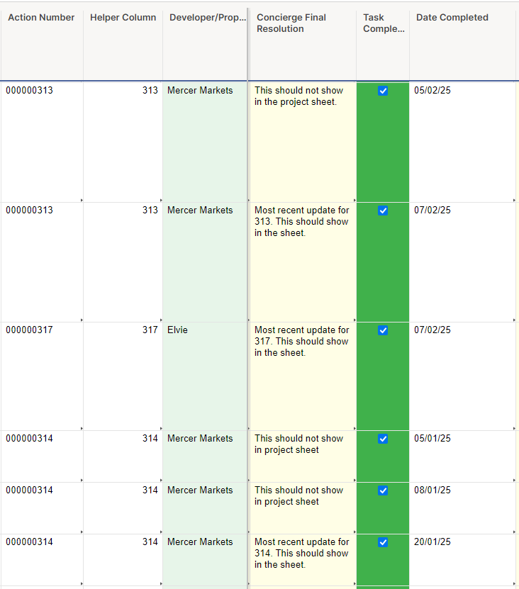
Here is a pic of the Completed Action sheet:

I want to latest comment from the 6/2 in the Concierge Final Resolution column to show in the partner sheet for project/action number 000000312 (Project 1)
If anyone could help me I would be soooooo grateful, I have spent far too long on trying to get this already!!! I am desperate!!!!