SHow Availability based on Bookings

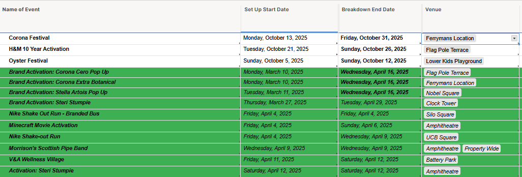
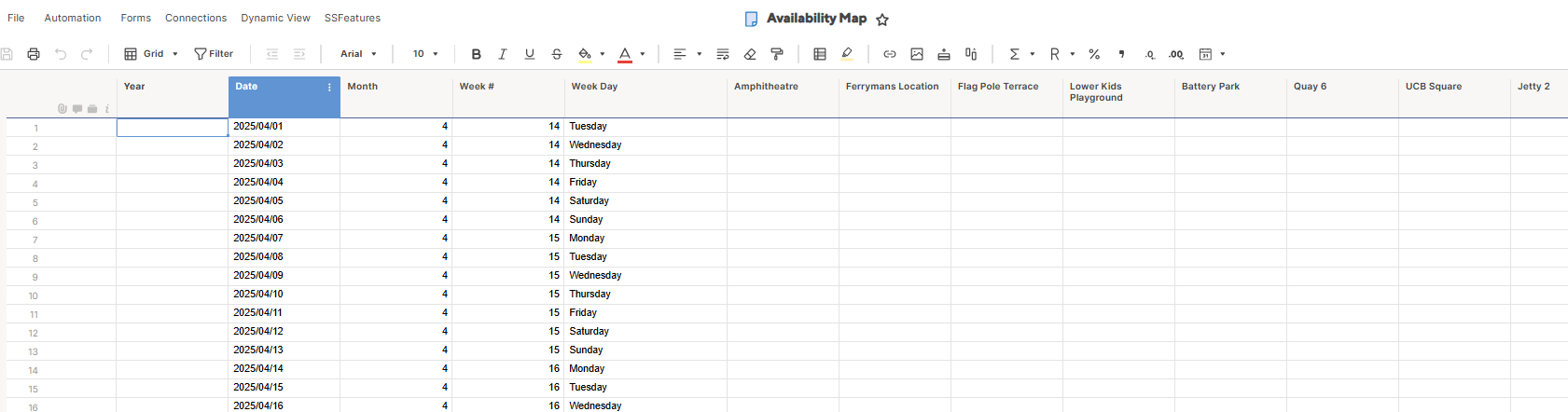
I have two sheets, the primary is the booking sheet that has the event dates both start and end date, venue, client details etc. This would be my reference sheet. I have created another sheet that shows the availability of all the venues based on confirmed bookings per venue this is my Availability Sheet.

Teh venue in teh reference sheet are select from drop down list. In the Availability Sheet I will create a column for each venue. For the sake oif example the firts venue is Amphitheatre

I am battling to create a formula that doesn't give me a UNPARSABLE. I started with this:

=IFERROR(INDEX({Event_Name_Ref}; MATCH(1; ({Venue_Ref}=@column )*({Start_Date_Ref}<=[Date]@row )*({End_Date_Ref}>=[Date]@row ); 0)); "Available")

The { } reference from the reference sheet only and no reference from the Availability Sheet.

Is this formula correct for EU?

Is this the right kind of formula?

My Availability Sheet has a row for each day of the year. I want to show across all veneus what is booked and where

PLease can you help me.

Find more posts tagged with

Accepted answers

Paul Newcome

You will need different formulas for each of the venue columns, but it is a very easy tweak to the base formula for each.

=JOIN(COLLECT({Source Sheet Event Column}, {Source Sheet Start Date Column}, @cell <= Date@row, {Source Sheet End Date Column}, @cell >= Date@row, {Source Sheet Venue Column}, HAS(@cell, "Amphitheatre")), CHAR(10))

There near the end where it is "Amphitheatre" is where you would change it for each of the different venue columns in the target sheet.

All comments

Paul Newcome

Are you able to provide some screenshots for context?

GeorgeM

Thanks for responding Paul.

The first grab in green this is the source sheet - the one below is the one I am creating.

Essentially, the source sheet is a ive working document that every enquiry and booking we get goes onto this sheet, it include a lot of dtail like costs, client details etc.

The Availability Map, is something I am trying to create that pulls from this sheet that if I needed to look high level at all the venues on our property ona particular day it would show which one had a booking - the event name can be inserted and perhaps the cell changed to a color automatically and if available can just say available and remain white.

I would also like to ensure if ont he source sheet a booking is removed that it automatically removes from the availability map.

I plan to then create a dashboard that shows this ina visual format

Paul Newcome

You will need different formulas for each of the venue columns, but it is a very easy tweak to the base formula for each.

There near the end where it is "Amphitheatre" is where you would change it for each of the different venue columns in the target sheet.

GeorgeM

Thanks Paul, this worked perfectly.

I wanted ot add a condition that when one of the cells within a column have a booking that cell changes colour. I went to conditional formating but it only seems to highlight the entire columns or entire rows when in fcat i just want to highlight the cell that has a value.

Is this possible?

Paul Newcome

It will not highlight the entire column. It will be applied to the entire column but only highlight rows that meet the criteria of the rule. You can also select within the rule which column(s) get highlighted when the criteria is met.

https://help.smartsheet.com/learning-track/level-2-workflows/conditional-formatting

GeorgeM

Is there a way to highlight only the cell that has a value? If a cell contains a formula, Smartsheet considers it not truly blank, even if the formula returns an empty string (""). So when you set a conditional formatting rule like “Cell is not blank,” it will still highlight that cell — because technically, the formula makes it non-blank.

How can I work around this?

Sign in to join the conversation!

Quick Links

Component react.discussion.discussions had an error.

ref must be one of: categoryID, siteSectionID, category, category/categoryID, category/name, category/description, category/url, category/allowedDiscussionTypes, locale, siteSection, siteSection/basePath, siteSection/contentLocale, siteSection/sectionGroup, siteSection/sectionID, siteSection/name, siteSection/description, siteSection/apps, siteSection/attributes, layoutViewType, discussionID, commentID, page, sort, discussion, discussion/name, tags, breadcrumbs, discussionApiParams, serverDraftID, serverDraft.