Pulling a distinct list with conditions

Karenmst

Hi,

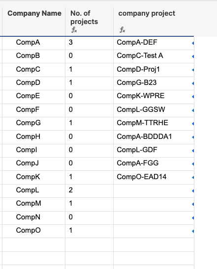
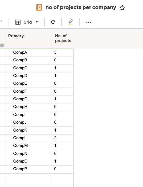
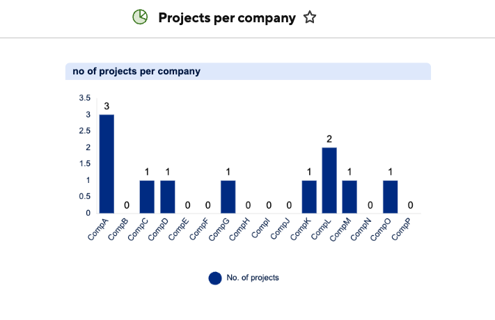
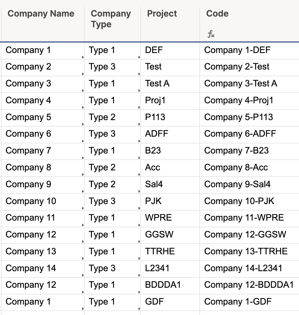
I have an equation that works to pull a list of distinct entries in to sheet 1 from a column in a different sheet (sheet 2). I would now like to add some conditions to what items are pulled into my list, based on information contained in sheet 2. The equation that works with no conditions is:

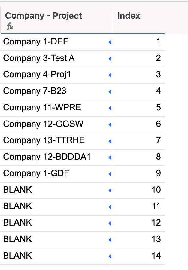
=IFERROR(INDEX(DISTINCT({Sheet 2 - Company Name}), Index@row ), "BLANK")

The condition I would like to add, is to only pull Company Name if the 'Company Type' is 'Type 1'.

Your help is much appreciated! Thanks

Georgie

Hi @Karenmst,

We can adjust your existing formula to use the COLLECT Function - this allows us to collect values that meet multiple criteria. Using it with DISTINCT will mean only distinct values are returned. Give this a try:

• =IFERROR(INDEX(DISTINCT(COLLECT({Sheet 2 - Company Name}, {Sheet 2 - Company Type}, "Type 1")), Index@row ), "BLANK")

Does that work for you?

Georgie

Karenmst

Hi Georgie,

Thank you! That works! I have a follow up question for you:

My sheet 1 (Company summary sheet) will be dynamic, because the Companies listed in Sheet 2 (Company project data) and the conditions will change from time to time. The way I have set up this equation using the index row, requires that I pre-populate the index row (I have currently populated 100 rows with the numbers 1-100). This assumes that I will have <100 company names on my summary sheet (sheet 1) at any given time. Currently I only have ~ 20, which means all of the other rows are just listed as 'BLANK'. But this gives space for the list to be dynamic as the Sheet 2 data changes.

Is there a better way that I should have set this up to pull a Distinct list Companies from the sheet 2 (project data sheet) which can list a company multiple times if they have multiple projects?

Ultimately, I would like to graph the data in Sheet 1 (E.g. Company name vs # of projects), but not yet sure on how to set up the graph if the number of rows in Sheet 1 will be dynamic.

Appreciate any additional insights you may have. Thanks in advance.

Georgie

Hi @Karenmst,

Glad to hear that works!

To make sure that you can have the same company name listed more than once in your Company Summary Sheet (sheet 1) when they have more than one project, you could create another column in your Company project data sheet (sheet 2) that uses a formula to concatenate the company name and the project name.

For example, your formula might be:

• =[Company Name]@row + "-" + Project@row

Or, if you’d rather have a shorter code, you could use the LEFT Function to take only a certain number of characters from either or both columns, such as in the following examples - you can use however many characters you'd like from each column: 

• =LEFT([Company Name]@row , 4) + "-" + Project@row
• =LEFT([Company Name]@row , 5) + "-" + LEFT(Project@row , 3)
• =[Company Name]@row + "-" + LEFT(Project@row , 3)

Once you have your concatenated company name and project code, you could then adjust the formula you use in sheet 1 to use that column as the column that’s pulled through, so your formula would be:

• =IFERROR(INDEX(DISTINCT(COLLECT({Sheet 2 - Code}, {Sheet 2 - Company Type}, "Type 1")), Index@row ), "BLANK")

I tested this on my end and confirmed that the formula correctly pulls through only companies where the type is Type 1, and only rows where the code (company name + project name) are distinct. 

As you can see, the formula still uses your index column. You could, however, use an auto-number column (see Auto-number rows) as your Index column so that every new row in sheet 1 will be automatically populated with the next number in the sequence.

So, your sheet 2 may look something like this:

And your sheet 1 could look something like this:

Hope that helps!

Georgie

Karenmst

Hi Georgie,

Thank you for your effort to help solve my question! The way you've mocked up Sheet 2 is very accurate, and I have already set up a 'Project Unique ID' column (equivalent to your Code column). But what I am trying to do in Sheet 1 (Summary sheet) would be to only list each Company once and then count the number of projects they have. So my sheet 1 is currently set up with columns: Index, Company Name, # of projects, (+ some columns for additional summary metrics that are collected with COUNTIF or SUMIF equations to pull data from sheet 1 by referencing Company Name@row).

So sheet 2 is currently working correctly thanks to your 1st response! But my second question(s) are:

1. Is there a way to accomplish what we've built in sheet 2 without having 80 rows of 'BLANK' (e.g. was there another way of doing this without the INDEX equation and needing to reference the Index column)? This question is only educational for me to understand if there was a more efficient way for me to have built this.
2. Now that I have sheet 1 built and showing a list of company names + number of projects per company - how do I graph this data? With the understanding that new companies could be added to the list at any time as sheet 2 is updated (e.g. any new companies added to sheet 2 will populate into sheet 1 in a row currently filled with BLANK). My corporate dashboard needs a graph showing a list of all the companies we are supporting graphed by the number of projects per company - but of course I don't want a graph that includes 80 rows of BLANK!

Any ideas? Thanks!

Georgie

Hi @Karenmst,

We can adjust your formula so that we don’t need the Index column by using the MATCH Function. This will output the same results as the formula in my previous response. However, you can also change the “BLANK” section to “” so that where there’s no match, it displays a blank cell. Your formula in the summary sheet would therefore be:

• =IFERROR(INDEX(DISTINCT(COLLECT({Sheet 2 - Code}, {Sheet 2 - Company Type}, "Type 1")), MATCH([Company Name]@row , {Sheet 2 - Company Name}, 0)), "")

Your summary sheet would then look something like this:

As you can see, I have now added a column that counts the number of projects each company has (my formula counts  how many times the company name in each row appears in the company project column). 

In order to create a chart that will include all new entries, without having to manually edit the chart each time a row is added, you can create a row report using your summary sheet as the source.

In the same workspace, click Create > Report > Row Report, and name your report as desired (for example “Number of projects per company”. In the report, select your summary sheet as the source sheet, and then select the Company Name (this may be the primary column, which is added by default) and your # of projects column. Your report should then look similar to this:

This report will then be automatically updated whenever new rows are added or any changes are made to your summary sheet. We can therefore use this report as the source for a chart on a dashboard.

In a dashboard, create a chart widget and select your report as the source. Reports are charted in their entirety, which is why we only want to include the company name column and the number of projects column in the report. You can then select the chart type and customise the chart as desired. As an example, here’s what your chart could look like:

Does that work for you? Happy to help with any further questions!

Georgie

Paul Newcome

If you are trying to graph the companies with the number of projects for each, you can simply create a row report that references the source sheet, group it by company, then use the summarize feature to get the count. You can then use that report to create your chart.

You can skip the summary sheet(s) completely.