Showing trends for continuously updating data sheet

Mohammed Sulaiman

I'm trying to create a trend indicator (Down, Sideways, Up) from a sheet, which has columns - Created Date "Tasks", "Expected % Complete"," Complete %", and a helper column "% Complete %/Expected % Complete" ratio.

What formula to use, to compare values " Complete %/Expected % Complete" ratio, for the last and penultimate entries based on the Created Date Columns.

Example : if the last entry of the task "REDUCE DEFICIENCIES AT COMPLETION BY 25% BY FYE" has a higher "Complete %/Expected % Complete" ratio, than the penultimate entry, return "Up".

if the last entry of the task "REDUCE DEFICIENCIES AT COMPLETION BY 25% BY FYE" has the same "Complete %/Expected % Complete" ratio, than the penultimate entry, return "Sideways".

if the last entry of the task "REDUCE DEFICIENCIES AT COMPLETION BY 25% BY FYE" has a lower "Complete %/Expected % Complete" ratio, than the penultimate entry, return "Down".

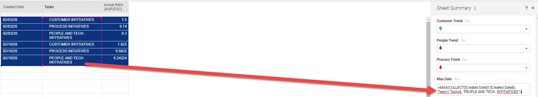
This formula is to be shown in the sheet summary.

Genevieve P.

Hi Mohammed,

Although this sounds pretty simple, because of the variables in your sheet we will need to create a number of different formulas to end up with the final result. The first thing to do is to be able to indicate which entry is the last one for that specific task, and which entry is the penultimate. Once we've figured out what those two dates are, then we can run a bigger formula to find the difference between the rows with those dates and the specific task name.

1 . MAX Date

First, you'll need two additional Summary Fields to return the most recent entry and the penultimate entry. To fine the most recent entry, we'll use a MAX(COLLECT formula, like so:

=MAX(COLLECT([Created Date]:[Created Date], Tasks:Tasks, "REDUCE DEFICIENCIES AT COMPLETION BY 25% BY FYE"))

2 . Penultimate Date

This will return the largest (or newest) date for that task. Then we can use this to find the penultimate date for that task by excluding this MAX date in the next formula. In my sheet I've named the summary field "Latest Date: Reduce Deficiences":

=MAX(COLLECT([Created Date]:[Created Date], [Created Date]:[Created Date], <>[Latest Date: Reduce Deficiencies]#, Tasks:Tasks, "REDUCE DEFICIENCIES AT COMPLETION BY 25% BY FYE"))

3 . Finding the Values with JOIN(COLLECT

Now that you have the Latest date and the Penultimate date for these columns, you can use these references to create your Nested IF statement. In order to have the formula read the value in your Complete%/Expected% column, we will need to use a JOIN(COLLECT formula to return the value if the Created Date is the Latest One and if the Task name is correct:

JOIN(COLLECT([Complete%/Expected%]:[Complete%/Expected%], [Created Date]:[Created Date], [Latest Date: Reduce Deficiencies]#, Tasks:Tasks, "REDUCE DEFICIENCIES AT COMPLETION BY 25% BY FYE"))

Then we have to compare this to the same value, but referencing the Penultimate date, instead:

JOIN(COLLECT([Complete%/Expected%]:[Complete%/Expected%], [Created Date]:[Created Date], [Penultimate Date: Reduce Deficiencies]#, Tasks:Tasks, "REDUCE DEFICIENCIES AT COMPLETION BY 25% BY FYE"))

4 . Nesting the values into the IF statement

Now that we know how to return the two values, we can create our statement with the IF and the Symbols. This next statement will look crazy, but it's just adding in the relation between those two formulas above... Greater Than ( >), Equal To (=), or Less Than (<).

Try this in your Status field:

=IF(JOIN(COLLECT([Complete%/Expected%]:[Complete%/Expected%], [Created Date]:[Created Date], [Latest Date: Reduce Deficiencies]#, Tasks:Tasks, "REDUCE DEFICIENCIES AT COMPLETION BY 25% BY FYE")) > JOIN(COLLECT([Complete%/Expected%]:[Complete%/Expected%], [Created Date]:[Created Date], [Penultimate Date: Reduce Deficiencies]#, Tasks:Tasks, "REDUCE DEFICIENCIES AT COMPLETION BY 25% BY FYE")), "Up", IF(JOIN(COLLECT([Complete%/Expected%]:[Complete%/Expected%], [Created Date]:[Created Date], [Latest Date: Reduce Deficiencies]#, Tasks:Tasks, "REDUCE DEFICIENCIES AT COMPLETION BY 25% BY FYE")) = JOIN(COLLECT([Complete%/Expected%]:[Complete%/Expected%], [Created Date]:[Created Date], [Penultimate Date: Reduce Deficiencies]#, Tasks:Tasks, "REDUCE DEFICIENCIES AT COMPLETION BY 25% BY FYE")), "Sideways", IF(JOIN(COLLECT([Complete%/Expected%]:[Complete%/Expected%], [Created Date]:[Created Date], [Latest Date: Reduce Deficiencies]#, Tasks:Tasks, "REDUCE DEFICIENCIES AT COMPLETION BY 25% BY FYE")) < JOIN(COLLECT([Complete%/Expected%]:[Complete%/Expected%], [Created Date]:[Created Date], [Penultimate Date: Reduce Deficiencies]#, Tasks:Tasks, "REDUCE DEFICIENCIES AT COMPLETION BY 25% BY FYE")), "Down")))

Let me know if you have any questions about this!

Cheers,

Genevieve

Mohammed Sulaiman

Hi Genevieve,

I get an error, saying invalid column value at step 1.

I have simplified the columns and data in it for the sake of this exercise, with the same logic. For any task, the latest Actual Ratio should be greater than penultimate entry, for trending "Up" for that particular task. Latest Actual Ratio less than Penultimate Entry for trending "Down". If no change, then "Sideways".

Example : Customer Trend is Up, based on the Actual Ratio comparison of the latest and penultimate entry.

The second part to this question is:

The above process is manual for data entry, where the ratio will need to be entered every week.

However when an automated function was used to "copy only parent rows" from one sheet to another, the child rows were also copied.

Is there a way to copy only parent rows from one sheet to another. The objective is to get a snapshot of how the task is performing, week over week, without getting into the details of child rows.

Once the weekly actual ratio is collected for the tasks, the first part comes into play, which is showing the trend in the sheet summary of the copied sheet.

Thanks,

Genevieve P.

Hi Mohammed,

It looks like you're entering this formula into a Text/Number field, but it would need to be a Date Type field, so it can return the Max Date.

In regards to your second question, about copying parent rows, it sounds like you might want to create a report instead (see here). You can edit information from Reports (users will need to be shared to the report and the source sheets as an Editor or higher).

To do this, you could include a helper column in your sheet that checks a box if the row is a Parent or not. Then, the Report Criteria could look for that checkbox and pull through any rows that are a Parent. This means that the Report will continually update as new Parent rows are created, for that easy overall snap-shot.

Here's the formula that will looks to see if a row is a Parent row:

=IF(COUNT(CHILDREN(Tasks@row)) >= 1, 1, 0)

It says, if the count of Children rows (in the column "Tasks") is greater than or equal to 1, then check the box.

Let me know if this will work for your purposes.

Cheers,

Genevieve

Mohammed Sulaiman

Thanks Genevieve,

Got the first part to work and it looks like below, and working as it should.

I also agree that the reports let you pull the parent level information only. However with the reports, how do I get the above outcome. The report keeps updating itself based on the current date, and doesn't have historical data.

Say for example, today is Feb 17th, in my report, I'll only have information pertaining to Feb17th, and not Feb 3rd, 10th.

Is there a way to show historical data in a report as well.

My original thoughts were to use automated copy over function and copy only the parent level tasks to a different sheet at fixed intervals. And the trends are calculated in the sheet summary of that sheet, as seen above.

The only challenge is the child rows also being copied, which just skews the data in the sheet, is there a workaround while copying over.

Genevieve P.

Glad to hear the first part is working!

The data that is shown in your report will depend on what criteria you have set up for it. Can you post a screen capture of your report with the report builder open? From there we should be able to adjust what rows are showing up - both historical and present.

If you wanted to just create copies, then you would still need to create the "Parent checkbox" helper column to check whether or not a row is a Parent. Then the trigger for your workflow would be if the box is checked. Does that make sense? I can provide some screen capture examples if needed.