Text to columns vs IF statement

cnikkih

I have daily report that contains a string of text (Reasons) regarding issues that occurred overnight. These are usually anywhere from 2 to 20 in each report, and while that is manageable on a day to day basis, I'm trying to pull in the last year's worth of data and that is entirely too much to parse by hand.

I'd like to be able to copy those Reasons into a Smartsheet and have it then automatically do a "Text to Columns" function. I used the following formulas so far:

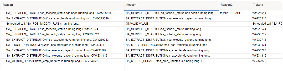
For Reason1: =LEFT(Reason@row, FIND("CW#", Reason@row) - 1)

For Ticket#: =RIGHT(Reason@row, LEN(Reason@row) - FIND("CW#", Reason@row))

1. In the Reason1 field now, when the expected text to find is not there, it gives an "#INVALID VALUE" message, and puts the entire string in the Ticket# field. What needs to happen is that the string should be in Reason1 and nothing should be in Ticket#.
2. In the Ticket# field, even though I selected CW# as the qualifier, it only uses C, leaving W# in the Ticket field. I would just use # but that symbol gets used in other parts of the string sometimes, so it is not a valid qualifier. Nor is just C or W for obvious reasons. Does Smartsheet only allow a single character here, or is there a way to get it to identify a set of characters? "CW#" appears to work in the formula for Reason1, because in most of the reasons, there is a C long before CW# appears, so I would assume it would split the string at the first C.
3. The Reason2 field was my attempt to write another formula to correct the issue where #INVALID VALUE shows up the Reason1 field... I was thinking that if I had to, I could write something that basically says "If Reason1 is Invalid, use the test from the Reason field. So far, I wrote =IF(AbendTemp@row = "#INVALID VALUE", " "), AbendTemp@row but Nested IF statements still confound me, so I'm not surprised to find it doesn't work. I also really don't want to have yet another formula column to try to pull out this info. I'd prefer to be able to handle it in a single function if possible, combined with the current formula I'm using in the Reason1 field.

Have I confused everyone enough? And is this even feasible? Hopefully the image helps.

Paul Newcome

Try using an IFERROR function on the first formula.

=IFERROR(LEFT(........................), Reason@row)

And for the ticket #, we can add 2 to the output of the FIND function like so:

=RIGHT(Reason@row, LEN(Reason@row) - (FIND("CW#", Reason@row) + 2))

cnikkih

This is so helpful! I have not used IFERROR before. Still have a couple of questions but this is so much better.

The columns shown below are Reason, Reason1, and Ticket#. Reason1 is still not displaying anything if the expected text string "CW#" is not found in the line. Instead, it is showing the text under Ticket#. In the image below, lines 1-3 & 5 are pretty much correct, except it is leaving a C at the end. Not the end of the world, but it would be nice if it was gone. But for lines 4, 6, & 7... everything in the first column should also display in the second, and nothing should be in the third.

Paul Newcome

My apologies. It isn't the IFERROR that we want. We want an IF instead for the Reason.

=IF(FIND("CW#", Reason@row) = 0, Reason@row, LEFT(Reason@row, FIND("CW#", Reason@row) - 1))

For the ticket number... The reason rows 4, 6, and 7 are displaying as they are is because the symbol # is missing. There is no "CW#" for the FIND function to grab.