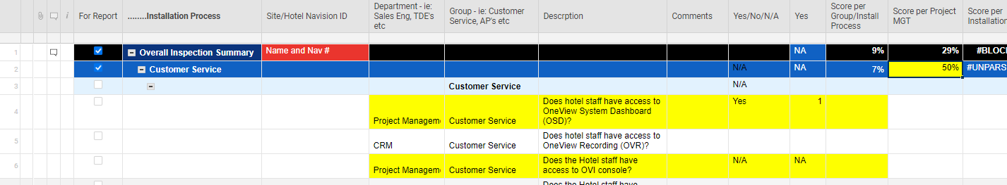
Countifs not calculating as expected

Whenever I change a field to NA it should exclude counting it into the average but it is not doing that. It is staying at 50% but should be 100%. Please let me know what I need to do. See screen shot.
=(SUM(Yes4, Yes6)) / ((COUNT([Department - ie: Sales Eng, TDE's etc]4, [Department - ie: Sales Eng, TDE's etc]6)) - (COUNTIFS(Yes4, "NA", Yes6, "NA")))
Thank you.
Comments
-
COUNTIFS is looking for both criteria, not either. I think you need to use COUNT with OR:
=(SUM(Yes4, Yes6)) / ((COUNT([Department - ie: Sales Eng, TDE's etc]4, [Department - ie: Sales Eng, TDE's etc]6)) - (COUNT(OR(Yes4 = "NA", Yes6 = "NA")))) -
Hi thanks for your suggestion! I just had to tweak it to look like this in order for it to calculate however
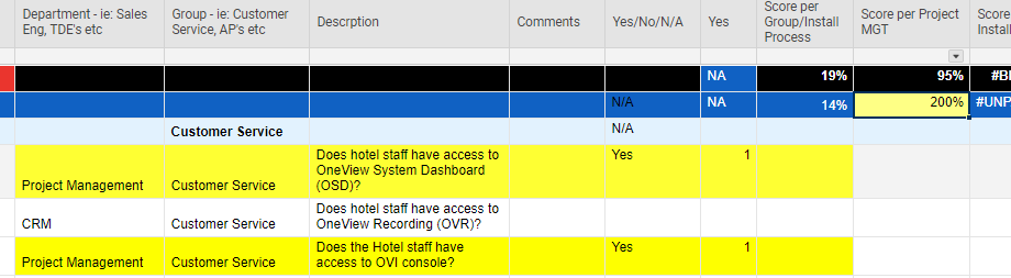
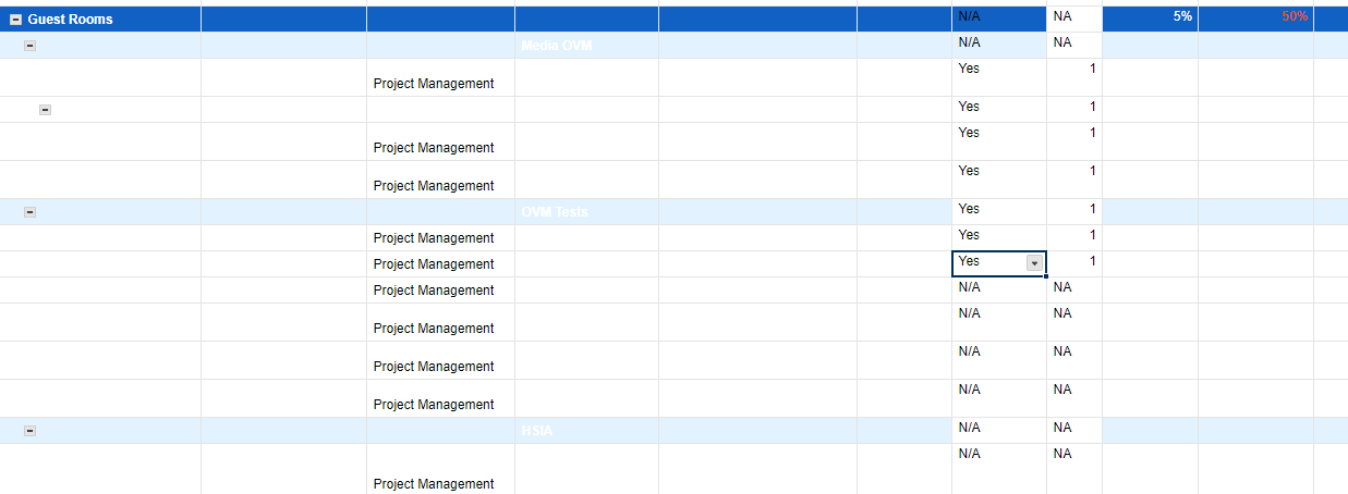
1. when I select both questions to answer Yes , I get 200% where I only want 100%. The N/A portion works though.
=(SUM(Yes4, Yes6)) / ((COUNT([Department - ie: Sales Eng, TDE's etc]4, [Department - ie: Sales Eng, TDE's etc]6) - (COUNT(OR(Yes4 = "NA", Yes6 = "NA"))))) (pic attached)
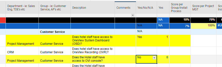
2. when I select 1 yes and 1 no I need to see 50% whereas the results 100% (pic attached)
I need it to score only on yes and no answers and when NA is selected it makes sure not to average into the equation.
any thought would be great. This has been very trying. :-(
-
Right. I'm not sure that COUNT/OR combination is even functioning correctly. Rather than doing the whole calculation, could you simply use AVG to average the cells with numbers:
=AVG(Yes4, Yes6)
That will average only numbers and ignore NA entries.
-
If you do need to use your original formula, I think you would have to do it this way:
=(SUM(Yes4, Yes6)) / (COUNT([Department - ie: Sales Eng, TDE's etc]4, [Department - ie: Sales Eng, TDE's etc]6) - (COUNTIF(Yes4, ="NA") + COUNTIF(Yes6, ="NA")))
-
You could also try something along the lines of
=SUM(CHILDREN(Yes@row)) / COUNTIFS(CHILDREN(Yes@row), ISNUMBER(@cell))
This will sum the range up (which only looks at numbers anyway), then divide it by how many cells in the range contain a number (leaves out the N/A's).
Using the CHILDREN function also allows the addition or deletion of rows without having to worry about whether or not a range within a formula needs adjusted.
-
I like the Children idea however not sure it will work. I need scored Averages per Department of which there are several in the Department column...so I need to select only those departments ie: Project Management which are shatter through the 300 questions.
-
This might work! I will give this a try now and let you know. Thank you very much
-
Ah. Ok. Then this...
=SUMIFS(Yes:Yes, [Department - ie: Sales Eng, TDE's etc]:[Department - ie: Sales Eng, TDE's etc], "Project Management") / COUNTIFS(Yes:Yes, ISNUMBER(@cell), [Department - ie: Sales Eng, TDE's etc]:[Department - ie: Sales Eng, TDE's etc], "Project Management")
This will look at the entire column and only calculate for those that have the department as Project Management. Just replace the underlined portion with whatever department you are wanting to calculate for.
-
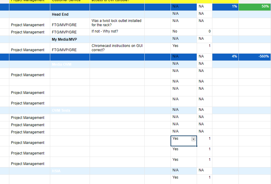
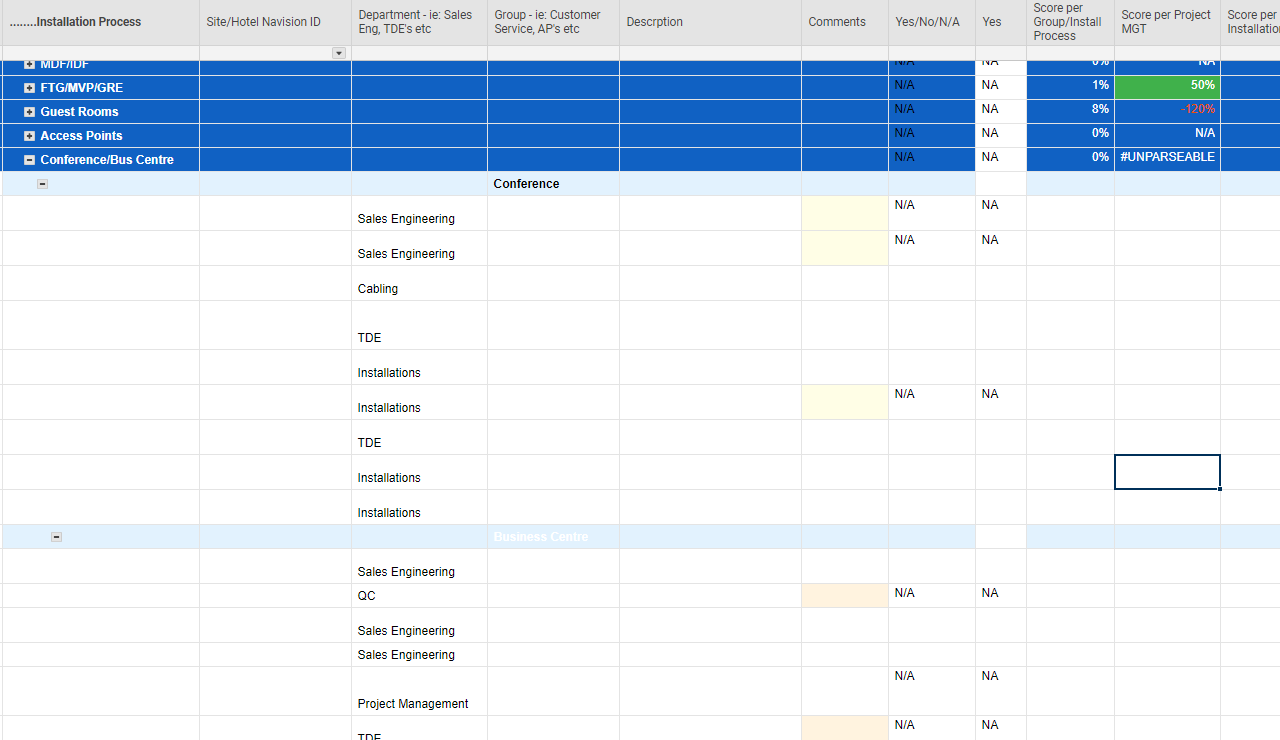
This is bizarre. The first 2 sections work fine with your formula. did not count the NA and scored correctly.
However for the next larger section, I am getting negative scores whenever I select NA. After changing them all the NA is gave me a -1000%. Any ideas would be appreciated. :-)
=SUM(Yes183, Yes206, Yes208, Yes228, Yes229, Yes230, Yes250, Yes252, Yes263, Yes291) / COUNT([Department - ie: Sales Eng, TDE's etc]183, [Department - ie: Sales Eng, TDE's etc]206, [Department - ie: Sales Eng, TDE's etc]208, [Department - ie: Sales Eng, TDE's etc]228, [Department - ie: Sales Eng, TDE's etc]229, [Department - ie: Sales Eng, TDE's etc]230, [Department - ie: Sales Eng, TDE's etc]250, [Department - ie: Sales Eng, TDE's etc]252, [Department - ie: Sales Eng, TDE's etc]263, [Department - ie: Sales Eng, TDE's etc]291) - (COUNTIF(Yes183, ="NA") + (COUNTIF(Yes206, ="NA") + (COUNTIF(Yes208, ="NA") + (COUNTIF(Yes228, ="NA") + (COUNTIF(Yes229, ="NA") + (COUNTIF(Yes230, ="NA") + (COUNTIF(Yes250, ="NA") + (COUNTIF(Yes252, ="NA") + (COUNTIF(Yes263, ="NA") + COUNTIF(Yes291, ="NA"))))))))))
-
To use the above formula, you will need to wrap the last bit in parenthesis. The basic order of operations is parenthesis, multiplication, division, addition, subtraction. Following this order, you are dividing the sum by the count THEN subtracting the N/A's. Try this formula. Not the added parenthesis after the / and at the end of the formula...
=SUM(Yes183, Yes206, Yes208, Yes228, Yes229, Yes230, Yes250, Yes252, Yes263, Yes291) / (COUNT([Department - ie: Sales Eng, TDE's etc]183, [Department - ie: Sales Eng, TDE's etc]206, [Department - ie: Sales Eng, TDE's etc]208, [Department - ie: Sales Eng, TDE's etc]228, [Department - ie: Sales Eng, TDE's etc]229, [Department - ie: Sales Eng, TDE's etc]230, [Department - ie: Sales Eng, TDE's etc]250, [Department - ie: Sales Eng, TDE's etc]252, [Department - ie: Sales Eng, TDE's etc]263, [Department - ie: Sales Eng, TDE's etc]291) - (COUNTIF(Yes183, ="NA") + (COUNTIF(Yes206, ="NA") + (COUNTIF(Yes208, ="NA") + (COUNTIF(Yes228, ="NA") + (COUNTIF(Yes229, ="NA") + (COUNTIF(Yes230, ="NA") + (COUNTIF(Yes250, ="NA") + (COUNTIF(Yes252, ="NA") + (COUNTIF(Yes263, ="NA") + COUNTIF(Yes291, ="NA")))))))))))
-
I copied but got UNPARSEABLE. :-(
I need all yes and no answers to be averaged per Installation Process, in this case 'Conference parent... for department "Project Management"
=SUMIFS(Yes:Yes, [Department - ie: Sales Eng, TDE's etc]:[Department - ie: Sales Eng, TDE's etc], "Project Management") / COUNTIFS(Yes:Yes, ISNUMBER(@cell), [Department - ie: Sales Eng, TDE's etc]:[Department - ie: Sales Eng, TDE's etc], "Project Management")
-
Hi Paul
I applied this however I change all the answers to Yes which provided 100% Great! But then I changed 5 out of the 10 answers to = NA. the score went down to 50% and needs to remain 100% because we do not want those NA calculated into the scores.
-
Try the below formula. It should simplify things greatly for you...
=SUMIFS(Yes:Yes, [Department - ie: Sales Eng, TDE's etc]:[Department - ie: Sales Eng, TDE's etc], "Project Management") / COUNTIFS(Yes:Yes, ISNUMBER(@cell), [Department - ie: Sales Eng, TDE's etc]:[Department - ie: Sales Eng, TDE's etc], "Project Management")
You are summing the Yes column if the department column = (in this example) Project Management. You are then dividing it by how many cells in the Yes column contain a number and are in the same row where the department is (in this example) Project Management.
-
Sorry I didn't have your formula in there . I put this one in but get Unparseable.
=SUM(Yes183, Yes206, Yes208, Yes228, Yes229, Yes230, Yes250, Yes252, Yes263, Yes291) / (COUNT([Department - ie: Sales Eng, TDE's etc]183, [Department - ie: Sales Eng, TDE's etc]206, [Department - ie: Sales Eng, TDE's etc]208, [Department - ie: Sales Eng, TDE's etc]228, [Department - ie: Sales Eng, TDE's etc]229, [Department - ie: Sales Eng, TDE's etc]230, [Department - ie: Sales Eng, TDE's etc]250, [Department - ie: Sales Eng, TDE's etc]252, [Department - ie: Sales Eng, TDE's etc]263, [Department - ie: Sales Eng, TDE's etc]291) - (COUNTIF(Yes183, ="NA") + (COUNTIF(Yes206, ="NA") + (COUNTIF(Yes208, ="NA") + (COUNTIF(Yes228, ="NA") + (COUNTIF(Yes229, ="NA") + (COUNTIF(Yes230, ="NA") + (COUNTIF(Yes250, ="NA") + (COUNTIF(Yes252, ="NA") + (COUNTIF(Yes263, ="NA") + COUNTIF(Yes291, ="NA")))))))))))
-
Your formula above has too many parenthesis in it. Try this version...
=SUM(Yes183, Yes206, Yes208, Yes228, Yes229, Yes230, Yes250, Yes252, Yes263, Yes291) / (COUNT([Department - ie: Sales Eng, TDE's etc]183, [Department - ie: Sales Eng, TDE's etc]206, [Department - ie: Sales Eng, TDE's etc]208, [Department - ie: Sales Eng, TDE's etc]228, [Department - ie: Sales Eng, TDE's etc]229, [Department - ie: Sales Eng, TDE's etc]230, [Department - ie: Sales Eng, TDE's etc]250, [Department - ie: Sales Eng, TDE's etc]252, [Department - ie: Sales Eng, TDE's etc]263, [Department - ie: Sales Eng, TDE's etc]291) - COUNTIF(Yes183, ="NA") + COUNTIF(Yes206, ="NA") + COUNTIF(Yes208, ="NA") + COUNTIF(Yes228, ="NA") + COUNTIF(Yes229, ="NA") + COUNTIF(Yes230, ="NA") + COUNTIF(Yes250, ="NA") + COUNTIF(Yes252, ="NA") + COUNTIF(Yes263, ="NA") + COUNTIF(Yes291, ="NA"))