Formula to Calculate Percentage Change from Baseline

wispsofsmoke

Hi,

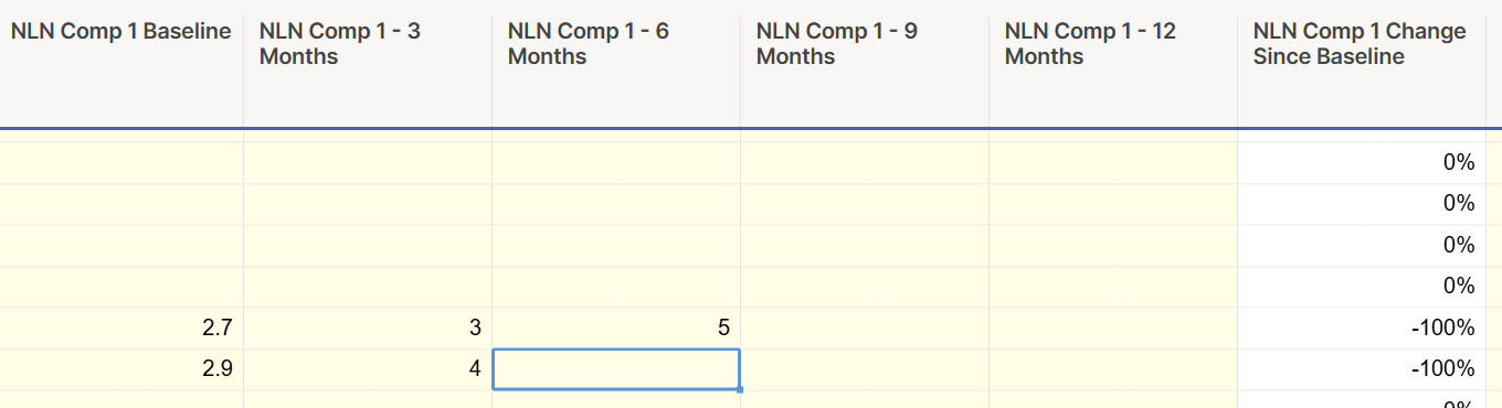
We capture scores between 1-5 each month. I'm looking to create a formula to calculate the percentage change from the baseline based on the most recent month's entry in that row.

For example, baseline (starting) score was 3 in June (captured in the column "June"). Let's say it's now August and the score is 4 (captured in the column "August"), so I want a "Percentage Change" column to show 33%, representing the change from June-August. When a score is entered for September, I want the "Percentage Change" column to automatically show the percentage change between June-September.

Thanks in advance!

Paul Newcome

Try this update. It looks like my fingers and brain weren't working together very well on that.

=IFERROR((INDEX(COLLECT([First Column]@row:[Last Column]@row, [First Column]@row:[Last Column]@row, @cell <> ""), COUNTIFS([First Column]@row:[Last Column]@row, @cell <> "")) - [Baseline Column]@row) / [Baseline Column]@row, "")

ChristianFinke

@wispsofsmoke

To calculate the percentage change from the baseline, use a formula like =IF([June]@row = 0, 0, ([Last Column Name]@row - [June]@row) / [June]@row * 100), replacing [Last Column Name] with the most recent month’s column. If columns change often, a helper column could track the latest score dynamically.

wispsofsmoke

Thanks Christian!

Is there a way to have it scan for the most recent column automatically so I don't have to update the month name?

For example, I want to have placeholder columns for each month per year vs. add new columns each month and then have the "Percentage Change" column at the end (to the right, after December). So, let's say I already have columns in 2024 for June through December. If I enter a score today for November, it would calculate the change from June-November, but the December column would be blank. When I enter a score in the December column, it would then update for June-December because there is now data in that column.

Is that possible? I know I've done it in Excel but don't remember how.

wispsofsmoke

Hi,

Still not quite getting this to work correctly. Attaching a screenshot of my table. This is the formula in the last "NLN Comp 1 Change Since Baseline" column:

=IF([NLN Comp 1 Baseline]@row = 0, 0, ([NLN Comp 1 - 12 Months]@row - [NLN Comp 1 Baseline]@row) / [NLN Comp 1 Baseline]@row * 1)

At some point, I'll have data in the -9 and -12 Month columns. I just want it to look first in the 12 Month column and then, if blank, keep looking left until it finds a populated column and calculate the percentage between that right-most column and the baseline.

For example, for the row that shows 2.7 in the "NLN Comp 1 Baseline" column and 5 in the "NLN Comp 1 - 6 Months" column, I want it to show the percentage change between the 5 and the 2.7 in the "NLN Comp 1 Change Since Baseline" column. Then, when I enter a number in the "NLN Comp 1 - 9 Months" column, I want the percentage change to automatically calculate that percentage change in the "NLN Comp 1 Change Since Baseline" column instead. So, the "NLN Comp 1 Change Since Baseline" column will always calculate the percentage change between the "NLN Comp 1 Baseline" column and the right-most column that has a number.

Thanks!

Paul Newcome

@wispsofsmoke Try this:

=IFERROR((INDEX(COLLECT([First Column]@row:[Last Column]@row, [First Column]@row:[Last Column]@row <> ""), COUNTIFS([First Column]@row:[Last Column]@row, @cell <> "")) - [Baseline Column]@row) / [Baseline Column]@row, "")

The above should allow you to not have to keep changing the formula each time data is entered into the next column as time goes on. It should automatically pull the rightmost column that has data entered and the compare it to the baseline.

wispsofsmoke

@Paul Newcome I tried using the formula but get an #INCORRECT ARGUMENT SET error. Any ideas?

I tried both with the original column names and then with renaming the columns to match your formula exactly (First Column, Last Column, Baseline Column).

Thanks!

Paul Newcome

Try this update. It looks like my fingers and brain weren't working together very well on that.

=IFERROR((INDEX(COLLECT([First Column]@row:[Last Column]@row, [First Column]@row:[Last Column]@row, @cell <> ""), COUNTIFS([First Column]@row:[Last Column]@row, @cell <> "")) - [Baseline Column]@row) / [Baseline Column]@row, "")

wispsofsmoke

@Paul Newcome that worked! Thanks Paul - I see your solutions on here often and appreciate your generosity and expertise!

Paul Newcome

Happy to help. 👍️