Issue with transcribing a reference formula for Add-On Rates

Lydia Bowman

Hi,

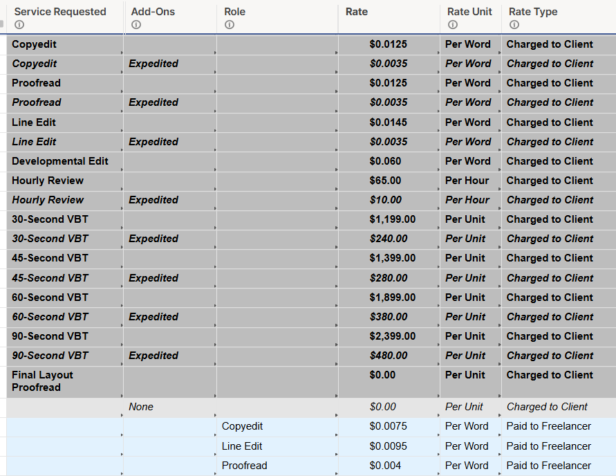
I'm having an issue with writing a reference formula for Add-On Rates. I've included pictures of the Reference Sheet and the Main Project Tracker here, with Client Name info redacted.

The "Team Member Rate Sheet Pull" helper and "Project Rate Sheet Pull" helper columns both have formulas that work:

Team Member: =IF(ISTEXT(Status@row), INDEX(COLLECT({Rate}, {Client Name}, [Client Name]@row, {Role}, Status@row), 1))

Project Rate: =IF(ISTEXT(Status@row), INDEX(COLLECT({Rate}, {Client Name}, [Client Name]@row, {Project Type}, Status@row), 1))

What I have tried so far for Add-On Rate Sheet Pull that is giving incorrect values or #INVALID VALUE errors:

=IF(ISTEXT([Add-Ons]@row), INDEX(COLLECT({Rate}, {Client Name}, [Client Name]@row, {Add-Ons}, [Add-Ons]@row), 1))

=IF(ISTEXT([Status]@row), INDEX(COLLECT({Rate}, {Client Name}, [Client Name]@row, {Add-Ons}, [Add-Ons]@row), 1))

Thanks in advance for any help!

Jgorsich

With this formula you are collecting ALL the add-ons for a given company that match that name ("Expedited") and then choosing the first one. For these customers, I presume you have expedited proofread AND expedited hourly review available - and if you choose the first one there is no certainty that you'll choose the one you intend.

Add, to your collect() formula, a criteria for your "Service Requested" and you'll probably be good.

Jgorsich

#Invalid Value is an interesting result (Formula error messages | Smartsheet Learning Center). It seems to be trying to tell you that it isn't finding any data to collect.

You may be trying the formula on a row that is particularly unlucky (I've done this before), or it may be that your Client Names and Addon Names are slightly different between the two sheets. Try making it a column formula first to catch the "Unlucky row" scenario, then pick a single example and make sure that the data matches EXACTLY - this is sometimes easiest by using simpler formulas to troubleshoot, like countifs() or even just countif() to check 1 criteria at a time.

Lydia Bowman

Hi @Jgorsich,

Thanks for the note! That's helpful.

Lydia Bowman

Follow up note/question here:

I was able to work out some of these issues, but I'm still having an issue with this formula pulling incorrect information in (see highlighted examples attached).

These should be pulling in $280 and $10, respectively. I've written the formula this way:

=IF(ISTEXT([Add-Ons]@row), INDEX(COLLECT({Rate}, {Client Name}, [Client Name]@row, {Add-Ons}, [Add-Ons]@row), 1))

Thanks for any further thoughts or assistance!

Jgorsich

With this formula you are collecting ALL the add-ons for a given company that match that name ("Expedited") and then choosing the first one. For these customers, I presume you have expedited proofread AND expedited hourly review available - and if you choose the first one there is no certainty that you'll choose the one you intend.

Add, to your collect() formula, a criteria for your "Service Requested" and you'll probably be good.

Lydia Bowman

Thanks, that did the trick!