Risk Score Formula

Karl86

Hi Im looking for some help please.

In for my Project Raid Log I would like a formula based on risk score to show the following symbols

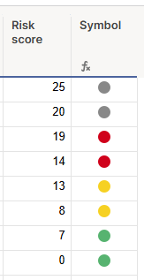
Risk score of 25 - 20 - Black

Risk score of 19 -14 - Red

Risk Score 13 - 08 - Amber/Yellow

Risk Score of 0 -7 - Green

Thanks in advanced.

Nick Korna

Hi @Karl86,

A nested IF should take care of this for you:

=IF([Risk score]@row >= 20, "Gray", IF([Risk score]@row >= 14, "Red", IF([Risk score]@row >= 8, "Yellow", "Green")))

Sample output:

I've used "Gray" here as I can't see a symbol set with black, but if needs be just substitute the relevant value in place in the formula.

Hope this helps, but if I've misunderstood anything or you've any problems/questions then just let us know!

Karl86

Hi Nick,

This is perfect thank you for this. Sorry forgot to add if we can have formula if risk score is blank can we show as N/A please?

Many thanks

Karl86

Thanks @Nick Korna

This is perfect thank you for this. Sorry forgot to add if we can have formula if risk score is blank can we show as N/A please?

Nick Korna

Hi @Karl86,

Amended slightly to give N/A if score is blank (but another cell in the row is filled in):

=IF([Risk score]@row >= 20, "Gray", IF([Risk score]@row >= 14, "Red", IF([Risk score]@row >= 8, "Yellow", IF([Risk score]@row <> "", "Green", "N/A"))))

If nothing else in the row has anything in, then this will be blank.

Karl86

@Nick Korna thanks ahh ok so we have the below so maybe if we could have a formula that only calculates risk score for entries that are risks only under type column?

Nick Korna

@Karl86,

Sure - what is the source/formula for your risk score?

For example, if it's something simple like Impact Score + Likelihood Score then it'd be:

=IF(Type@row = "Risk", SUM([Impact Score]@row:[Likelihood Score]@row), "")

If you have more details, then can help amend this to what you require.

Karl86

@Nick Korna thanks yeah its impact score + likelihood score so for example impact score is 5 and likelihood score is 5 would give a raid score of 25..

As we also store issues and actions on our raid log we would like to only produce the RAG symbols for risks only

Nick Korna

IF(AND) is your friend here:

=IF(AND(Type@row = "Risk", [Risk score]@row >= 20), "Gray", IF(AND(Type@row = "Risk", [Risk score]@row >= 14), "Red", IF(AND(Type@row = "Risk", [Risk score]@row >= 8), "Yellow", IF(Type@row = "Risk", "Green", "N/A"))))

Sample output:

If you want to skip the Risk Score, you can:

=IF(AND(Type@row = "Risk", ([Impact Score]@row * [Likelihood Score]@row) >= 20), "Gray", IF(AND(Type@row = "Risk", ([Impact Score]@row * [Likelihood Score]@row) >= 14), "Red", IF(AND(Type@row = "Risk", ([Impact Score]@row * [Likelihood Score]@row) >= 8), "Yellow", IF(Type@row = "Risk", "Green", "N/A"))))

Sample output:

The Risk Score 2 is just showing what the numbers are to save some maths - you wouldn't need it in an actual sheet.

Hope this helps, but let me know if I've misunderstood something or you've any problems/questions.