Is there a way to create 2 Reports from one Sheet with different formatting?

BTO84

I am looking to create 2 Reports from one Sheet that contains employee time off requests. The Sheet contains 13 columns, but for simplicity, the relevant fields are as follows:

Employee Name
Division
Start Date
End Date
PTO Used (# of hours)
Approved?

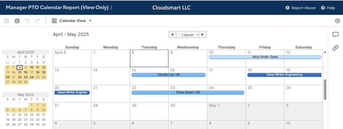
I would like to have one report for the managers to show Name, Division, Start, End, and Approved. I want it to color code by Division so each manager has a view of all divisions but can pick theirs out at a glance. Also it would be viewed in Calendar View with each entry titled in the format of "Name - Division". Unapproved requests would be filtered out of this report.

The second report would be for payroll to show Name, Start, End, PTO, Approved. This should be color coded by the Approved column so they can focus on the approved requests normally, but still have visibility of the unapproved requests in case employees are asking why PTO wasn't used. This would also be viewed in Calendar View with each entry titled in the format of "Name - PTO Used".

I already know how to set up a calendar view to show each request as a time range using the Start and End fields. And in a Sheet, I know how to do conditional formatting and how to create formulas to combine data from two columns into one phrase. I've read that I'll probably need to create formula columns in the original Sheet to create the names I want to see, but I'm new to Reports so I can't figure out how to use those columns as the Primary for the Report or apply conditional formatting.

jmyzk_cloudsmart_jp

Hi @BTO84

You're right that in Smartsheet, Calendar View coloring is set at the sheet level, not at the report level. Because of that, if you need two different color schemes (Division for managers vs Approval Status for payroll), here's a clean method:

First, it's important to know:

• Calendar View colors are based on the Primary Column.
• A sheet can only have one Primary Column, which means you can't change the Calendar display title between two different reports if they are both built from the same sheet.
• Also, Copy Row automation only moves the row once — it doesn't keep the two sheets synced if the original changes later.

Because of this, the best solution is to create a second sheet and link the data between them using cross-sheet formulas, not just copying rows.

Here’s the step-by-step:

In your Original Sheet:

• Add a System Column (Auto-Number type) called "Row ID".
• This automatically gives every row a unique ID automatically.

https://app.smartsheet.com/b/publish?EQBCT=49930dc8ef2e43aca9b73744c5116fbd

Create a second sheet for Payroll:

• Copy the sheet structure (Save as New) to keep the same columns.
• In the second sheet, use cross-sheet formulas to pull live data from the original sheet into the necessary columns, matching by the Row ID.
• Set the Primary Column differently if needed (for example, use "Name - PTO Used" as the title in the second sheet).

https://app.smartsheet.com/b/publish?EQBCT=97a46ea3912f48bb90fa2e3b64247bd9

Now you can apply separate Calendar View setups:

• In the Original Sheet, apply conditional formatting based on the Division for the Manager Calendar.
• In the Payroll Sheet, apply conditional formatting based on the Approval Status for the Payroll Calendar.

Finally, build two reports:

Manager PTO Calendar Report (based on the Original Sheet): Title is "Name - Division", colored by Division.

https://app.smartsheet.com/b/publish?EQBCT=ff0748ef86fa496b80d55b44b8db1dc3

Payroll PTO Calendar Report (based on the Payroll Sheet): Title is "Name - PTO Used", colored by Approval Status.

https://app.smartsheet.com/b/publish?EQBCT=b603b8e7149e4771815eff1234c64b9c

This way, each Calendar View is independent, the formatting fits the audience, and any updates to the original data automatically flow through to the second sheet using cross-sheet formulas — without having to manually recopy rows or set up complicated automations.

Formulas

[Name - Divistion] =IFERROR(INDEX({sample_time_off_requests_original Name-Divison}, [Row ID]@row), "")

[Start Date] =IFERROR(INDEX({sample_time_off_requests_original : Start Date}, [Row ID]@row), "")

[End Date] =IFERROR(INDEX({sample_time_off_requests_original : End Date}, [Row ID]@row), "")

[PTO Used (# of hours)] =IFERROR(INDEX({sample_time_off_requests_original : PTO Used}, [Row ID]@row), "")

[Approved?] =IFERROR(INDEX({sample_time_off_requests_original : Approved?}, [Row ID]@row), "")