SUMIFS - Sum, Restart, Sum Again

Hello Smartsheet Community!

I am trying to create a use a SUMIFS formula to add values in a column that are less than 20 within a 7 day range. Once they cross the threshold of 20, the formula should put a checkbox in the row that breached the threshold.

Next I want to repeat the process in successive rows, but ignore any rows used to cross the first threshold of 20.

I have a working formula for the first part, but I am uncertain how to accomplish the next phase.

Any suggestions would be helpful!

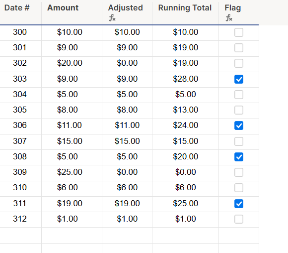
This is the working formula I have used that will yield the results in the chart below (date #s in the 100s). I am wanting an output that looks like the lower portion of the chart (date #s in the 200s).

=IF(SUMIFS(Amount:Amount, Amount:Amount, ABS(@cell ) < 20, [Date #]:[Date #], >=([Date #]@row - 6), [Date #]:[Date #], <=[Date #]@row) >= 20, 1, 0)

Find more posts tagged with

Formulas

Accepted answers

Mark.poole

@Andy_B

=IF(Amount@row >= 20, 0, Amount@row)

In the adjusted column treats any value 20 or over as a 0 for the purpose of the running total

=[Adjusted]1

for the first row in the running total column

=IF([Running Total]1 < 20, [Running Total]1 + Adjusted2, Adjusted2)

in the second row and dragged down to all the rest.

=IF([Running Total]@row >= 20, 1, 0)

For the flag column

All comments

Gia Thinh

Hi @Andy_B

Based on your description, I have made a simulation as shown below.

>20 column :

=IF(SUMIFS(Amount:Amount, Amount:Amount, ABS(@cell ) < 20, [Date #]:[Date #], >=([Date #]@row - 6), [Date #]:[Date #], <=[Date #]@row) >= 20, 1)

>20 excluded column :

=IF(AND([>20]@row = 1, COUNT(COLLECT([>20]:[>20], [>20]:[>20], 1, [Date #]:[Date #], >=([Date #]@row - 6), [Date #]:[Date #], <=[Date #]@row)) = 1), 1)

Is this what you want?

Andy_B

Hi @Gia Thinh,

Thanks for taking a crack at this! Unfortunately, I am still hitting some snags when I tried your suggestion. I created a new data set with consecutive days and this is what the formula produced:

The column on the right is what I am trying to accomplish with a formula. The logic would run something like this:

10 + 9 + 9 = 28 Cumulative sum is 20 or more, place a check ✔️ (Ignore Date # 302 - $20 or more)

Restart counting from zero

5 + 8 + 11 = 24 Cumulative sum is 20 or more, place a check ✔️

Restart counting from zero

15 + 5 = 20 Cumulative sum is 20 or more, place a check ✔️

Restart counting from zero

6 + 19 = 25 Cumulative sum is 20 or more, place a check ✔️ (Ignore Date # 309 - $20 or more)

Restart counting from zero

Let me know if you have any further thoughts!

Mark.poole

@Andy_B

I have done extensive research into your use case and Smartsheet can’t refer to the previous row’s value dynamically (@row - 1 isn’t supported). But you can manually configure each row’s formula once and drag it downward, so adding rows is easy, even if not fully automatic.

Mark.poole

@Andy_B The Solution I was able to come up with uses a few helper columns to achieve what your wanting. with a click and drag formula

Mark.poole

in the second row and dragged down to all the rest.

=IF([Running Total]@row >= 20, 1, 0)

For the flag column

Andy_B

Thank you @Mark.poole! I appreciate the insight - it's a tremendous help! I will be working the formulas and helper columns into my larger sheet. 😊

Sign in to join the conversation!

Quick Links

Component react.discussion.discussions had an error.

ref must be one of: categoryID, siteSectionID, category, category/categoryID, category/name, category/description, category/url, category/allowedDiscussionTypes, locale, siteSection, siteSection/basePath, siteSection/contentLocale, siteSection/sectionGroup, siteSection/sectionID, siteSection/name, siteSection/description, siteSection/apps, siteSection/attributes, layoutViewType, discussionID, commentID, page, sort, discussion, discussion/name, tags, breadcrumbs, discussionApiParams, serverDraftID, serverDraft.