How do I check an entire column for a particular value and only display the lowest example of it?

GCruz

The question title is kind of confusing, so here's what I'm looking to find out.

• I'm making a Project Plan sheet, and want to have a place that updates the estimated completion date based on how the project has progressed thus far.
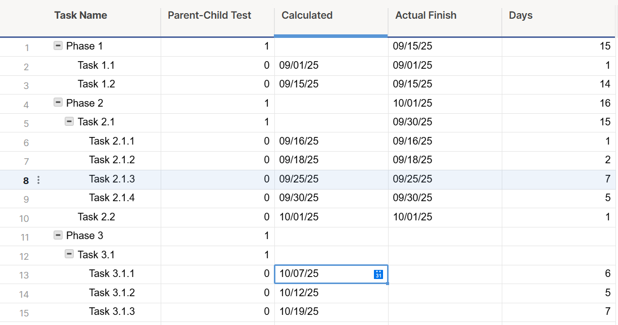
• There are more columns in my sheet, but my question is only related to the ones in the screenshot below.
• The screenshot below doesn't factor in WORKDAYS, but I'm not worried about that part. Once I understand the syntax of the formula I'm looking to create, I can add WORKDAYS in later.

I'll be using the formula in the [Calculated] column, and it will need to be a column formula. The logical flow I'm looking for is as follows:

1. Check if [Parent-Child Test]@row = 0
   1. If yes, go to #2
   2. If no, have [Calculated]@row = "" and then we're done
2. Check if [Actual Finish] <> ""
   1. If yes, have [Calculated]@row = [Actual Finish]@row ~and then we're done
   2. If no, go to #3
3. Check for the lowest row above @row that has [Parent-Child Test]@thatrow = 0
4. Have [Calculated]@row = SUM([Calculated]@thatrow + [Days]@row) ~and then we're done~

Basically, as the project progresses and tasks are completed, a user would enter the date that task was completed into the [Actual Finish] column. Then the rest of the unfinished tasks would update with a new projected finish date in the [Calculated] column based on when the task above it actually finished or is now estimated to finish. This would then auto-update a different cell that would display the new ETC date for the whole project (this last part I already know how to do using the MAX([Calculated]:[Calculated]) function).

So [Calculated]13 is 10/7/25 because it found the lowest row where [Parent-Child Test] = 0, row 10, and then added [Calculated]10 to [Days]13 to equal 10/7/25

Any help that you could provide would be greatly appreciated.

heyjay

Are you open to adding 2 helper columns?

1. RowNumber column, you can use AutoNumber.

2. Is Zero column that will check if the [Parent-Child Test]@row is Zero, if Yes, display the row number.

=IF( [Parent-Child Test]@row= 0, [RowNumber]@row, 0)

We can use this to index match the Days column using the formula.

=MAX([RowNumber]$1:[RowNumber]@row)