Reference the value of an active cell?

Is there a way to reference the value of an 'active cell value' in a formula or have a moving reference?

The current example code and screenshot specifically call out the desired outcome by referencing each cell in a range.

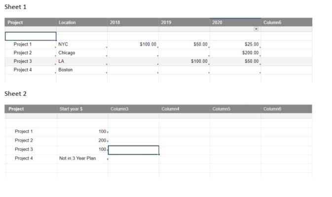
Example: Project1 will start in 2018, which is reflected on sheet 2.

formula in column 2 row 2 on sheet 2:

=IF(VLOOKUP(Project2, {SHEET 1 Range 3}, 3, false) > 0, {SHEET 1 Range 2}, IF(VLOOKUP(Project2, {SHEET 1 Range 3}, 4, false) > 0, {SHEET 1 Range 4}, IF(VLOOKUP(Project2, {SHEET 1 Range 3}, 5, false) > 0, {SHEET 1 Range 5}, "Not in 3 Year Plan")))

Is there a way I could get the formula to display the $ amount of the start year without specifically referencing each cell? I was looking to see if there was an 'active cell' type reference.

Example of thought:

=IF(VLOOKUP(Project2, {SHEET 1 Range 3}, 3, false) > 0, ActiveCell.value, IF(VLOOKUP(Project2, {SHEET 1 Range 3}, 4, false) > 0, ActiveCell.value, IF(VLOOKUP(Project2, {SHEET 1 Range 3}, 5, false) > 0, ActiveCell.value, "Not in 3 Year Plan")))

Any thoughts on this would be a great help. Thank you.

Find more posts tagged with

Formulas

Project Management

Cell linking

Comments

Paul Newcome

I feel like an INDEX/MATCH may have the flexibility you're looking for. Let me play around with it some, and I'll get back to you...

Are you trying to pull the EARLIEST year populated?

Update: If you are trying to pull the earliest year populated, you could use the following formula updating any cross-sheet references as needed of course.

=IFERROR(INDEX({Community Test Range 1}, MATCH(Project@row, {Community Test Range 2}, 0), COUNTIFS(INDEX({Community Test Range 1}, MATCH(Project@row, {Community Test Range 2}, 0)), ISBLANK(@cell)) + 1), "Not in 3 Year Plan")

See image below for testing of this particular solution.

Sean N

Yes, I am trying to pull the value from the EARLIEST year populated. Thanks!

Paul Newcome

Not sure if you saw it or not, but I have updated my original post with a solution. Hope it helps.

Sean N

Thanks! This looks helpful.

Just a question, what are the cell ranges for the references "Community Test Range 1" and Community Test Range 2"?

Paul Newcome

Oops. My apologies...

Range 1 is the year columns. Range 2 is the Project column.

Basically the way it all works is this...

The first portion of the INDEX function establishes where to pull the data from that you are wanting to display which would be your year columns.

The second portion of an INDEX function determines the row. For that we use a MATCH function to look for the Project Name.

The third portion is the column number which is where it got a little tricky. First we re-established the row with the original INDEX/MATCH as we did in parts one and two. Then we counted the number of blank spaces and added 1. This gave us the number of columns to move from left to right to pull the data from.

Sign in to join the conversation!

Quick Links

Trending discussions

Looking for assistance with a formula
Hi all, I am new to formulas and functions in Smartsheet and have a large sheet that I would like to summarize using an "average" formula/function. I need to include at least 2 separate criteria to filter correctly and I am having trouble combining the avg and collect functions as suggested in the functions list. I have…
Need help in formula function
I'm not able to get this formula to function in Smartsheet. The material ordered date is 9/3/2025. Am I missing something to get the date rage to populate? =TEXT([Material Ordered Date]@row +28,"MM/DD/YYYY")&"-"&TEXT([Material Ordered Date]@row +42, "MM/DD/YYYY")
I am trying to find a value in a table based on 2 criteria.
I am trying to find a value in a table based on 2 criteria. One of the values is dynamic from a drop down menu, while the other is static value in a column. The first value is found in column "Building type" and the other is found in Resource type. The table I am referencing is also shown. The result would be shown in the…