Validation Formula

Eric Tronson

Going crazy.

My current formula

=IF(AND([Time Missed / Used (In Hours)]1 < 19.99),CONTAINS("Not", [Excused/Not Excused]1:[Excused/Not Excused]1, ".25", "1"))) = #UNPARSEABLE

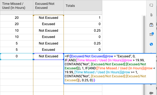
The goal here is to return .25 or 1 into a cell "Totals" if cell "Time Missed / Used (In Hours)]" is less than 19.99 and cell "[Excused/Not Excused]". Default value of cell "Totals" = 0.

IF cell "[Excused/Not Excused]" contains "excused" THAN cell "Totals" =0

IF cell "[Excused/Not Excused]" contains "Not" and cell "[Time Missed / Used (In Hours)" GREATER than 19.99, Cell "Totals" = 1

IF cell "[Excused/Not Excused]" contains "Not" and cell "[Time Missed / Used (In Hours)" is GREATER 1 but less THAN 19.99, Cell "Totals" = .25

Genevieve P.

Hi Eric,

It looks like you have kept the row reference in with your column names - you'll want to remove those to indicate a column range (instead of [Excused/Not Excused]1:[Excused/Not Excused]1, see [Excused/Not Excused]:[Excused/Not Excused] where I removed the 1s)

This formula would be broken down into your three different IF Statements:

1 . If the cell in this row is "Excused", return 0

=IF([Excused/Not Excused]@row = "Excused", 0

2 . If the time in this row is greater than 19.99, AND the Excused column contains "Not", then return 1

IF(AND([Time Missed / Used (In Hours)]@row > 19.99, CONTAINS("Not", [Excused/Not Excused]:[Excused/Not Excused])), 1

3 . If the time in this row is less than 19.99, but greater than or equal to 1, AND the Excused column contains "Not", return 0.25

IF(AND([Time Missed / Used (In Hours)]@row < 19.99, [Time Missed / Used (In Hours)]@row >= 1, CONTAINS("Not", [Excused/Not Excused]:[Excused/Not Excused])), 0.25

4 . Any other type of cell (ex. below 1), return 0

Once we add them all together, with the correct brackets, we get the following:

=IF([Excused/Not Excused]@row = "Excused", 0, IF(AND([Time Missed / Used (In Hours)]@row > 19.99, CONTAINS("Not", [Excused/Not Excused]:[Excused/Not Excused])), 1, IF(AND([Time Missed / Used (In Hours)]@row < 19.99, [Time Missed / Used (In Hours)]@row >= 1, CONTAINS("Not", [Excused/Not Excused]:[Excused/Not Excused])), 0.25, 0)))

Depending on how your columns are set up, you could actually trim this down and remove some of the extra rules, since Logic formulas read from left-to-right. It would be useful to see a screen capture of your sheet in grid view to help with this.

Here are some Help Center articles that may help as you build this: @row function / IF function / AND function / Column Ranges / Formula Creation tips

Let me know if you have any questions about this!

Cheers,

Genevieve

Genevieve P.

@Paul Newcome

= "criteria" should look for an exact match... no?

Great call on the @row!

Paul Newcome

@Genevieve P. I slipped on that one. My apologies. There were the other CONTAINS functions in the formula, plus other community posts already today using the CONTAINS function plus my own work today has been using CONTAINS a lot as well. I must be on CONTAINS overload. Haha.

I am still leaning towards the @row reference in the CONTAINS functions that are actually being used, but that is going to be something @Eric Tronson would need to weigh in on.

Genevieve P.

Hi Eric,

It looks like you have kept the row reference in with your column names - you'll want to remove those to indicate a column range (instead of [Excused/Not Excused]1:[Excused/Not Excused]1, see [Excused/Not Excused]:[Excused/Not Excused] where I removed the 1s)

This formula would be broken down into your three different IF Statements:

1 . If the cell in this row is "Excused", return 0

=IF([Excused/Not Excused]@row = "Excused", 0

2 . If the time in this row is greater than 19.99, AND the Excused column contains "Not", then return 1

IF(AND([Time Missed / Used (In Hours)]@row > 19.99, CONTAINS("Not", [Excused/Not Excused]:[Excused/Not Excused])), 1

3 . If the time in this row is less than 19.99, but greater than or equal to 1, AND the Excused column contains "Not", return 0.25

IF(AND([Time Missed / Used (In Hours)]@row < 19.99, [Time Missed / Used (In Hours)]@row >= 1, CONTAINS("Not", [Excused/Not Excused]:[Excused/Not Excused])), 0.25

4 . Any other type of cell (ex. below 1), return 0

Once we add them all together, with the correct brackets, we get the following:

=IF([Excused/Not Excused]@row = "Excused", 0, IF(AND([Time Missed / Used (In Hours)]@row > 19.99, CONTAINS("Not", [Excused/Not Excused]:[Excused/Not Excused])), 1, IF(AND([Time Missed / Used (In Hours)]@row < 19.99, [Time Missed / Used (In Hours)]@row >= 1, CONTAINS("Not", [Excused/Not Excused]:[Excused/Not Excused])), 0.25, 0)))

Depending on how your columns are set up, you could actually trim this down and remove some of the extra rules, since Logic formulas read from left-to-right. It would be useful to see a screen capture of your sheet in grid view to help with this.

Here are some Help Center articles that may help as you build this: @row function / IF function / AND function / Column Ranges / Formula Creation tips

Let me know if you have any questions about this!

Cheers,

Genevieve

Paul Newcome

Based on what I read in the post, I feel like maybe the CONTAINS functions should be using the @row reference instead of the column reference.

=IF([Excused/Not Excused]@row = "Excused", 0, IF(AND([Time Missed / Used (In Hours)]@row > 19.99, CONTAINS("Not", [Excused/Not Excused]@row)), 1, IF(AND([Time Missed / Used (In Hours)]@row < 19.99, [Time Missed / Used (In Hours)]@row >= 1, CONTAINS("Not", [Excused/Not Excused]@row)), 0.25, 0)))

I also agree that screenshots would be helpful though. If your [Excused/Not Excused] column contains either the option of "Excused" or "Not Excused", the above formula will never display anything other than 0 because "Not Excused" does contain the text of "Excused" which in turn causes the first IF to be true.

Genevieve P.

@Paul Newcome

= "criteria" should look for an exact match... no?

Great call on the @row!

Paul Newcome

@Genevieve P. I slipped on that one. My apologies. There were the other CONTAINS functions in the formula, plus other community posts already today using the CONTAINS function plus my own work today has been using CONTAINS a lot as well. I must be on CONTAINS overload. Haha.

I am still leaning towards the @row reference in the CONTAINS functions that are actually being used, but that is going to be something @Eric Tronson would need to weigh in on.

Eric Tronson

Thank you all! This helps tons I will let you know if this works!! This should close out my 2019 - 2020 Q1 goal!!!!

Paul Newcome

Happy to help! 👍️

Genevieve P.

Awesome! Let us know how it goes.

Eric Tronson

This worked perfectly. Thank you for the help. Love this community!

Genevieve P.

So glad to hear that! Thanks for the follow-up

Paul Newcome

Great!! This community is definitely a good one full of a ton of information.

Andrée Starå

This community is:

https://media.giphy.com/media/VDFoGg3JN1N4s/giphy.gif