Help with a SUMIF formula and a reconciliation spreadsheet

I am trying to build a reconciliation spreadsheet that compares two sets of data. Pictured below:

Screen Shot 2020-07-31 at 2.20.00 PM.png

The first set of data with the "QBO SKU" is pulling the information correctly using the below formula:

=SUMIFS({QBO – shipment history (7/30/20) Range 1}, {QBO – shipment history (7/30/20) Range 2}, Class@row, {QBO – shipment history (7/30/20) Range 3}, [QBO SKU]@row)

Screen Shot 2020-07-31 at 2.20.24 PM.png

The sheet it is referencing looks like this:

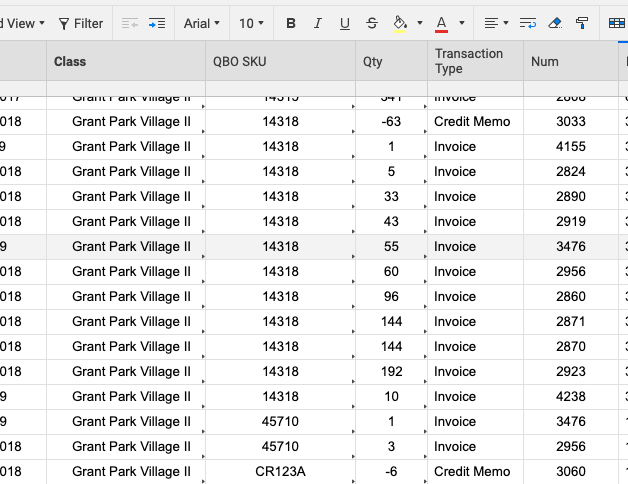
Screen Shot 2020-07-31 at 2.22.16 PM.png

The problem that I am running into is trying to replicate this successful formula for the second set of data.

I have copied the same formula and the same reference sheet layout but when I paste the code (pictured below) in the "Quantity" it is simply not calculating:

=SUMIFS({Podio – Shipment History Range 1}, {Podio – Shipment History Range 2}, Reference@row, {Podio – Shipment History Range 3}, [Podio SKU]@row)

Screen Shot 2020-07-31 at 2.25.28 PM.png

Furthermore, I have also included a "shipment type" column in the other reference sheet which I would like to pull in and calculate, because compared to the first data set ("QBO") this includes returns as well which affects the total count as it will determine if quantity needs to be added or subtract. Please see below for an example of the data I am trying to pull in:

Screen Shot 2020-07-31 at 2.27.36 PM.png

As you can see, we have "hardware shipment" which should be added up and "hardware return" which should be subtracted.

Just like the first formula, I would like to find out how many devices we shipped based off the unique SKU and whether it was a "shipment" or a "return".

From there, I'll be able to combine the two total quantities for each unique SKU in the "Total" column (far right) and successfully reconcile between the two sources of information.

Screen Shot 2020-07-31 at 2.30.35 PM.png

I also understand that this is quite dense to explain with screenshots, so if anyone in the community has some suggestions? I would be more than happy to connect over the phone and offer a more thorough explanation.

Thank you!

Find more posts tagged with

Accepted answers

Genevieve P.

Hi Mark,

First SUMIFS Question:

=SUMIFS({Podio – Shipment History Range 1}, {Podio – Shipment History Range 2}, Reference@row, {Podio – Shipment History Range 3}, [Podio SKU]@row)

The formula is built correctly and it's calculating, which to me indicates it's just not able to find a match for your two criteria (hence the 0 result). Can I ask how your Reference column in each sheet is populated? They would need to be letter-for-letter the exact same in order for this to calculate (including spaces before or after dashes - like this).

It would be helpful to see the full value in that Reference column in the sheet where the formula is, to make sure the values match.

Additionally, could you show the 3 references in that formula? (3 screen captures of what the pop-up window shows when you click the formula and choose edit reference over those 3 ranges). I just want to confirm it's looking in the right place for each value.

(See here for more information on Cross Sheet references).

Shipment Type:

In regards to the Shipment Type, are you looking for 2 calculations... one for if it was Shipped and one for if it was Returned? If so, you can build this out in the exact same way by simply adding another criteria to your SUMIF formula.

For example, this would SUM your Range 1 if the Class matches, the QBO SKU matches, and if the shipment type is Shipment:

=SUMIFS({QBO – shipment history (7/30/20) Range 1}, {QBO – shipment history (7/30/20) Range 2}, Class@row, {QBO – shipment history (7/30/20) Range 3}, [QBO SKU]@row, {Shipment Type column in other sheet}, "Property Hardware Shipment")

Then you could swap out the criteria for the other SUMIF statement:

You'd need to add in 2 columns to your calculation sheet though, one for each formula, if you needed both these results. Let me know if this works for you!

Cheers,

Genevieve

Genevieve P.

Almost there!

I wonder if the numbers are being read as Text instead of as numerical values?

Try adding a leading ' mark in front of the two numbers in the chart with the formula, like this:

'14318

'46562

You could also double click into one of the number cells in the source sheet to see if it contains a leading apostrophe. Are these manual entries?

All comments

Genevieve P.

Hi Mark,

First SUMIFS Question:

=SUMIFS({Podio – Shipment History Range 1}, {Podio – Shipment History Range 2}, Reference@row, {Podio – Shipment History Range 3}, [Podio SKU]@row)

It would be helpful to see the full value in that Reference column in the sheet where the formula is, to make sure the values match.

(See here for more information on Cross Sheet references).

Shipment Type:

For example, this would SUM your Range 1 if the Class matches, the QBO SKU matches, and if the shipment type is Shipment:

Then you could swap out the criteria for the other SUMIF statement:

You'd need to add in 2 columns to your calculation sheet though, one for each formula, if you needed both these results. Let me know if this works for you!

Cheers,

Genevieve

Mark Silvester

Thank you for your help Genevieve!

I can confirm that the Reference columns in each sheet are identical and I've included screen shots of the 3 references for the formula below:

Screen Shot 2020-08-04 at 3.30.01 PM.png

Screen Shot 2020-08-04 at 3.30.15 PM.png

Screen Shot 2020-08-04 at 3.30.33 PM.png

Please let me know if I can provide any extra information or screenshots.

The "Shipment Type" solution makes perfect sense as well thank you. :)

Genevieve P.

Hi @Mark Silvester

Ok so your formula is structured correctly and all the columns are set up exactly as they should be, which is great! Helps eliminate a few possibilities.

My next question is how you are getting the Quantity numbers that you're trying to SUM - is this being manually typed in (through a form or directly in the sheet), or are you using a formula to populate the Quantity column? (Range 1)

I'm wondering if it's somehow being read as text instead of as numerical values, which wouldn't be able to be Summed.

Thanks!

Genevieve

Mark Silvester

Hi Genevieve,

Thank you again for your help with this!

I can confirm that the quantity numbers have been manually typed in.

Screen Shot 2020-08-05 at 9.43.03 AM.png

Genevieve P.

Hi Mark,

This is going to take a little bit more digging... three more questions:

1 & 2 - How are the Reference and Podio SKU columns populated? (Also manual?)

3 - Can we do a test to confirm that the two Reference Columns really do have matching data?

Try this in a helper column in your destination sheet:

=COUNTIF({Podio – Shipment History Range 3}, Reference@row)

Essentially I'm just checking that if we do a cross-sheet formula looking into Range 3 that it can find a match to the values you have in the Reference column of your current sheet. If your COUNT returns 0, this indicates that the values aren't matching, and we'd want to look at how the Reference column is populated and make sure that the cells are letter-for-letter the exact same.

Let me know what you find out!

Cheers,

Genevieve

Mark Silvester

Success!

Thank you for your patience, Genevieve. After running the test it turns out the values weren't matching. Now that is fixed, I am finally pulling in some data!

That said, I was hoping you could help me figure out why SKU "14318" and "46562" are not calculating?

Screen Shot 2020-08-05 at 11.15.04 AM.png

Screen Shot 2020-08-05 at 11.16.02 AM.png

Thank you!

Genevieve P.

Almost there!

I wonder if the numbers are being read as Text instead of as numerical values?

Try adding a leading ' mark in front of the two numbers in the chart with the formula, like this:

'14318

'46562

You could also double click into one of the number cells in the source sheet to see if it contains a leading apostrophe. Are these manual entries?

Mark Silvester

Genevieve... you are a rock star!

This worked perfectly thank you! The sheet is now functioning just like intended.

Your help and patience has been very much appreciated.

Take care,

Mark

Genevieve P.

Wonderful!! Thanks for letting me know it worked!

I'm happy to have helped 🙂

Cheers,

Genevieve

Sign in to join the conversation!

Quick Links

Component react.discussion.discussions had an error.

ref must be one of: categoryID, siteSectionID, category, category/categoryID, category/name, category/description, category/url, category/allowedDiscussionTypes, locale, siteSection, siteSection/basePath, siteSection/contentLocale, siteSection/sectionGroup, siteSection/sectionID, siteSection/name, siteSection/description, siteSection/apps, siteSection/attributes, layoutViewType, discussionID, commentID, page, latest, sort, sortType, lookupSort, discussion, discussion/name, tags, breadcrumbs, discussionApiParams, serverDraftID, serverDraft.