Creating what seems to be a complicated report?

Tiara Rea-Palmer

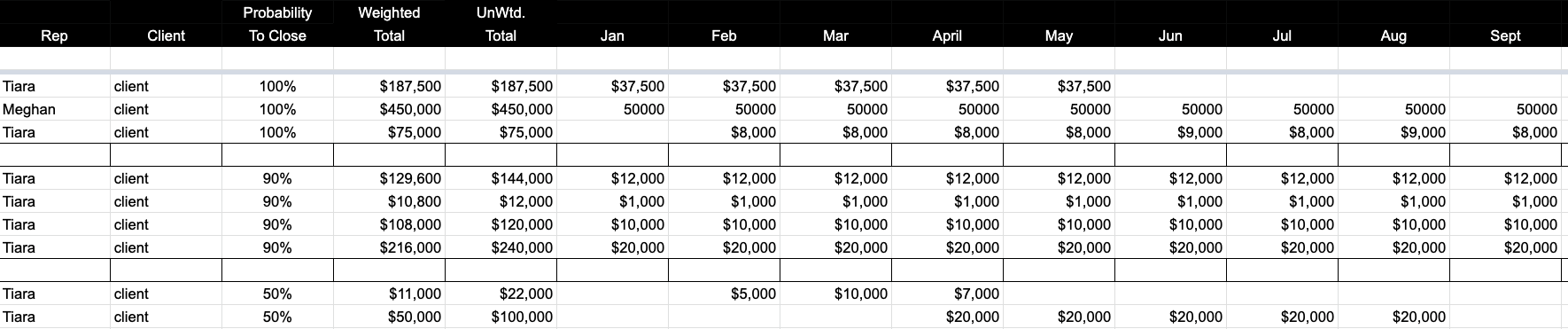
Trying to use the below as a template for a new report, but not sure if I can do so in SmartSheet or the best way to set it up.

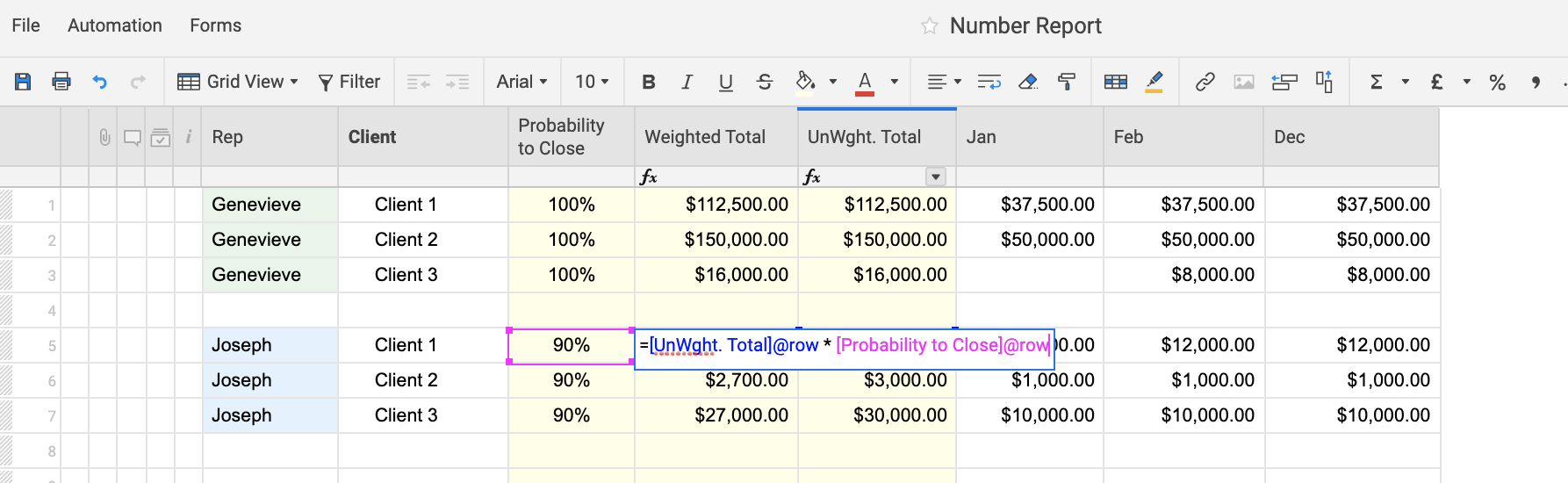
These are all fake numbers to start, but I'll want to pul them obviously from real numbers in other sheets and then group them by probability to close. Weighted total is based on probability, so at 90% closed, the Weighted Total should be 90% of that $ amount. The Unweighted Total is just the total, at 100%.

What's the best way to start this? Would it be best to create a new sheet and link cell #s? if so, how would I do the weighted and unweighted totals?

Or would a report be better? I tried that, but can't seem to figure out how to filter out duplicates (sometimes 1 client will book several different things under 1 package, but it only counts as 1 package even though there are multiple rows in SS).

Genevieve P.

Hi @Tiara Rea-Palmer

I would say that the way to do this will depend on how the information is stored in the other sheets, where you're pulling this information from.

You could definitely set up a sheet just like the one above in Smartsheet and then use formulas to calculate the weighted and unweighted totals, like so:

The formula above to create the unweighted total is

=SUM([First Column]@row:[Last Column]@row)

Then you would use this calculation with the Probability for the weight:

Here are some Help Center articles that you may find useful:

• SUM Function
• Create Efficient Formulas with @cell and @row
• Create a Cell or Column Reference in a Formula
• Set Formulas for All Rows with Column Formulas

Would this work for you? Are you wanting the data in the other columns (Jan/Feb/March, etc) to come from other sheets in Smartsheet? If so, it would be helpful to see screen captures of how this source data is housed, but please block out any sensitive data.

Cheers!

Genevieve

Tiara Rea-Palmer

Thank you! Those formulas worked great. Now I just need to figure out how to display the info housed in other sheets. Can you help with these as well?

Here's the headers I wound up creating:

I essentially need Merchant, Rep, Probability, and Months to be pulled from another sheet (sheet is called Placements Pipeline):

Merchant = Opportunity

Rep = Sales Rep

Probability = Probability

and Months (Jan, Feb, March, etc) come from the Month column

Genevieve P.

Hi @Tiara Rea-Palmer

My apologies for the delay! Were you able to figure out these formulas?

You would need to have a unique identifier for each row so that your second sheet knows which row to pull the data from... something to match the two rows together. Does that make sense?

@Paul Newcome has some great examples of formulas that can then use this unique identifier to pull data through. This post talks about unique identifiers. This post here goes through if you have multiple criteria to look for and match across sheets.

Tiara Rea-Palmer

Sadly, I'm not sure I understand. Is there a way you can help me in creating these formulas? And/or the unique identifiers?

Genevieve P.

No problem, I can definitely help create the formula, but it depends on your source sheet set up, the Pipeline. What makes each row in this sheet unique?

For example, is it the specific combination of different values that makes each row different? (So, this specific Merchant in combination with this specific Rep). Or is the Opportunity a value that is never repeated? (Could you have the same Opportunity value multiple times?) Or is there something else we can use, like an auto-number column that identifies each row?

I suppose the most important question is if you are looking to pull information across row-per-row (so just copying exactly what's in the other sheet) or if you need to combine data within the formula (such as Summing values in one column based on a criteria, like the Rep).

Genevieve P.

Here's an example of an INDEX(MATCH formula that uses the "Opportunity" column as a unique value that's in both sheets. This presumes that you have copied/pasted in or updated the sheet with the formula to have the same unique value.

This formula is to bring in the Rep's name:

=INDEX({Sales Rep Column}, MATCH(Merchant@row, {Opportunity Column}), 0)

Another idea would be to have a COPY ROW workflow set up from the first sheet to copy over a newly created row into the second sheet. Keep in mind this would be a copy/paste of the content so it wouldn't be linked or live. This means if you then updated the Sales Rep in the first sheet after the row had been copied it wouldn't change in the other sheet, does that make sense? Would copying the row get the information you need?

Tiara Rea-Palmer

What makes each row in Pipeline sheet unique? - There are no truly unique columns, as some Opportunities will repeat over time. So if I add a new column with auto-generated #, how would I do it in that case?

I suppose the most important question is if you are looking to pull information across row-per-row (so just copying exactly what's in the other sheet) or if you need to combine data within the formula (such as Summing values in one column based on a criteria, like the Rep). - I need to combine data within the formula, I believe.

Eventually, what I need to see is as follows:

Pulling live data from Placements Pipeline sheet

Merchant can have multiple Opportunities, but need them grouped. For example, RepA is 90% to closing 1 opportunity for MerchantA in Jan for $25,000 and 100% to 1 other opportunity in Feb for the same MerchantA for $10,000. Meanwhile, RepB closed an opportunity for MerchantZ for $9500 in Jan. So it would look something like this when done:

Does that make more sense?

Genevieve P.

Hi @Tiara Rea-Palmer

Yes, I think I understand a bit better now.

A Report may actually be the easiest way to go, then, since you can Group rows together and it can Sum this data based on criteria.

So, even if I have two Merchant A's, you can group by Merchant A. The duplicates would become child rows in the Report which you can minimize to see totals.

In this example, I have three rows for Client 2. I could minimize this to see a full row for Client 2 without all three rows beneath, like I've done for Client 1:

Is this closer to what you're looking for? The Report would be synced two-way, so you could update the data from the Report and it would update the sheet, and vice versa.

Tiara Rea-Palmer

Yes, I believe so!! I couldn't figure out how to do that in report-style through SS, but if that's easier, that would be great. It seems to still show all the info I'd need. How do I go about creating it?

Genevieve P.

Great! Let's try this then.

1. Create a Row Report
2. In the toolbar at the top, select your Source Sheet
3. Select all the columns you want populated in the Report
4. Group by Rep first, then by Merchant
5. Use the Summarize feature to roll up SUMs of each of the columns

I find it's easier to visually see how someone builds this out; please take a look at this Webinar which goes through the Grouping and Summary features: https://help.smartsheet.com/learning-track/best-practice-webinars/reports

Additionally, this Help Article has a brief video introduction to creating Reports, and a written step-by-step guide in regards to a Row Report: https://help.smartsheet.com/learning-track/smartsheet-intermediate/reports

Let me know if you have any questions or get stuck at any point when creating the Report after reviewing the links above and I'd be happy to help further! It would be useful to see a screen capture of how far you got in the Report.

Cheers,

Genevieve