Formula to change value to a number, then SUM

christine_ford2003

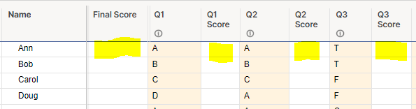
Hello! I am struggling with this formula & determined I need to start from the beginning. I have created a quiz. It is a mix of multiple choice (A,B,C,D) and True/False (T,F). Each letter will have a number value which is then SUM'd for a final grade. Something like this:

Question 1: A=5 / B=4 / C=3 / D=2

Question 2: A=0 / B=5 / C=3

Question 3: T=1 / F=0

Any suggestions?

Paul Newcome

Is there a reason you have different numbers for the same letter depending on the question? It would be MUCH easier if each letter was ALWAYS the same number. Otherwise you are going to have to rewrite the formula for every single row.

christine_ford2003

Thanks Paul! That is what I was afraid of.

Since the grade is determined by the highest score, if "A" was the same number (highest value), would mean "A" would have to always be the correct answer.

However, I am open to other options --- anything that could make this easier.

christine_ford2003

@Paul Newcome What if I have a separate sheet with the answer mapped to a value, something like this:

What is the formula to match the answer selected in the Primary sheet to the value assigned in the separate sheet?

Hope this made sense (??)

Paul Newcome

I think I misunderstood your original post. Regardless of the solution, you will need a separate formula for each column. Not a separate formula for each row.

If you were to create a table, the formula would look something like this...

=INDEX(COLLECT({Values Column}, {Question Column}, @cell = "Q1", {Answer Column}, @cell = [Q1]@row), 1)

You would just need to update both of the Q1 to Q2 or Q3.

If you did not want a table, you would use nested IF statements.

Q1 Score:

=IF([Q1]@row = "A", 5, IF([Q1]@row = "B", 4, IF([Q1]@row = "C", 3, IF([Q1]@row = "D", 2))))

Q2 Score:

=IF([Q1]@row = "A", 0, IF([Q1]@row = "B", 5, IF([Q1]@row = "C", 3)))

Q3 Score:

=IF([Q1]@row = "T", 1, 0)

Then you could add them all together to get the final score without needing a helper column for each:

=IF([Q1]@row = "A", 5, IF([Q1]@row = "B", 4, IF([Q1]@row = "C", 3, IF([Q1]@row = "D", 2)))) + IF([Q1]@row = "A", 0, IF([Q1]@row = "B", 5, IF([Q1]@row = "C", 3))) + IF([Q1]@row = "T", 1, 0)