Vlookup + sum in a column

christian.boza · 05/06/19

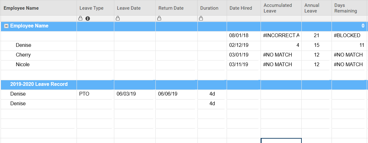
I am creating a template for keeping track of employee's leave. Column "Accumulated Leave" has the vlookup function to return the "leave days" taken by employees. the formula I have is as below:

=VLOOKUP([Employee Name]3, $[Employee Name]8:$Duration50, 5, true)

However, when I show the same employee on an another row, it does not sum up the total days of annual leave requested by the same employee.

Basically, I want to keep record of all leave requested throughout the year and deduct it automatically from the contract annual leave.

Thanks for the help!

Annotation 2019-05-06 181115.png

Paul Newcome · 05/06/19

Try using a SUMIFS instead of a VLOOKUP.

=SUMIFS(range_to_sum, criteria_range_1, criteria_1, criteria_range_2, criteria_2, .............)

christian.boza · 05/06/19

I had tried the sumifs formula as well, but i guess I did not do it right at first. Did not research this morning and used the one below:

=SUMIFS(Duration$8:Duration$50, [Employee Name]$8:[Employee Name]$50, "Denise")

and it worked just fine.

Thanks Paul.

Paul Newcome · 05/07/19

Happy to help.

A little tip regarding the SUMIF(S)...

They have very different syntax from each other. In SUMIF the range to sum is optional, and if you do want to specify, it comes last.

SUMIFS requires you to specify the range to sum and it comes first.

My recommendation and personal preference is to ALWAYS use the SUMIFS. You can use it with just one set of criteria range/criteria, and it will allow you to add additional criteria later if needed without having to change up the syntax completely.

(I also never use COUNTIF anymore either. Just COUNTIFS)

Vlookup + sum in a column

Comments

Help Article Resources

Categories