Find highest value and return matching column header

Isaac Gallardo · 12/17/20

Hi Everyone,

I have to inspect several cavities in a process by using a Smartsheet form. Then, out of this database, I would like to know the highest and lowest cavity weight along with the cavity #. I wonder how can I do that.

Here is an example:

If Cavity 2 has the highest value, and Cavity 1 has the lowest value. I would like to send out an email with the lowest cavity # and value, and the highest cavity # and value. Any idea on how to do that?

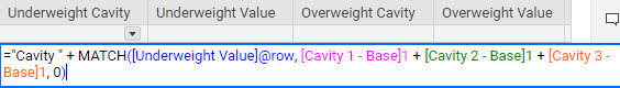
I figured that by creating 4 additional columns at the end of the file - (1) Underweight cavity, (2) Underweight Value, (3) Overweight Cavity, (4) Overweight value - could get this info then used these columns to set my email structure.

Email Structure: Cavity X has a value of XXX, and Cavity Y has a value of YYY.

Thank you for any help!

Paul Newcome · 12/17/20

I would start by using a MIN and a MAX function to pull the low and the high numbers.

=MIN([Cavity 1]@row:[Cavity 3]@row)

=MAX([Cavity 1]@row:[Cavity 3]@row)

Then you can use a MATCH function to pull the corresponding cavity number.

="Cavity " + MATCH([Underweight Value]@row, [Cavity 1]@row:[Cavity 3]@row, 0)

="Cavity " + MATCH([Overweight Value]@row, [Cavity 1]@row:[Cavity 3]@row, 0)

Isaac Gallardo · 01/15/21

Guys,

Thank you so much for your answers. But, I am still facing some issues with the sheet I am working on.

Each Cavity has three different inspections. If I have 3 cavities, the form will show:

Cavity - Shoulder

Cavity - Panel

Cavity - Base

I am only interested to obtain the weight variation on the base. So, I have something like this

Now, when I am trying to use the formula you gave me. it only shows Cavity 1 all the time. I think it is because the formula is applied to specific cells in the row and not to all rows. Any way to fix this.

Even if my underweight is located in Cavity 2. The formula shows Cavity 1. Any way I can fix this?

Paul Newcome · 12/17/20

I would start by using a MIN and a MAX function to pull the low and the high numbers.

=MIN([Cavity 1]@row:[Cavity 3]@row)

=MAX([Cavity 1]@row:[Cavity 3]@row)

Then you can use a MATCH function to pull the corresponding cavity number.

="Cavity " + MATCH([Underweight Value]@row, [Cavity 1]@row:[Cavity 3]@row, 0)

="Cavity " + MATCH([Overweight Value]@row, [Cavity 1]@row:[Cavity 3]@row, 0)

Mark Cronk · 12/17/20

Hi @Isaac Gallardo ,

Is this what you're looking for?

This will work if your cavities are number left to right in ascending order. You'll need to adjust the cavity range so that it includes all of your cavity columns:

Value [Underweight Cavity]: =MIN([Cavity 1]:[Cavity 3])

Value [Overweight Cavity]: =MAX([Cavity 1]:[Cavity 3])

Cavity # [Underweight Cavity]: =MATCH([underweight cavity]@row,[cavity 1]@row:[cavity 3]@row))

Cavity # [Overweight cavity]: =MATCH([overweight cavity]@row, [cavity 1]@row:[cavity 3]@row))

Work?

Mark

Isaac Gallardo · 01/15/21