Formulas for Calculating Time
Comments
-
thanks. but i also need the time in 24 hour format so that i can calculate duration
-
@Amanda P There are a number of solutions spread out throughout this thread that have conversions from 12 hour to 24 hour. The first step is pulling the hour (which it seems you had already accomplished). From there you would just need to pull the minutes, divide by 60, then add to the hours to get 11.25 for 11:25am or 23.5 for 11:30pm.
Once you get a number from the time, you can add/subtract as needed to get the duration, and there are a number of other solutions that will convert the number back into a time format.
-
An attempt at keeping as many of the solutions in this thread together as possible...
It is easier to convert the hours for 12 hour times to 24 hour times before attempting to do further calculations:
=VALUE(LEFT([Time Column]@row, FIND(":", [Time Column]@row) - 1)) + IF(CONTAINS("p", [Time Column]@row), IF(VALUE(LEFT([Time Column]@row, FIND(":", [Time Column]@row) - 1)) <> 12, 12), IF(VALUE(LEFT([Time Column]@row, FIND(":", [Time Column]@row) - 1)) = 12, -12))
this is just for the hour portion. The minutes portion would remain the same where we use
VALUE(MID(Timestamp@row, FIND(":", Timestamp@row) + 1, 2)) / 60
Calculating Time Worked for Employees
Can you calculate time in Smartsheet?
Conversion of timezones (Solved Formula Included)
Flagging a Date and Time Overlap
How do I create time of day columns?
Need to create a "shift" column from a time column
.
We needed to calculate how many WORKING hours were in between two dates/times.
Times are in 24 hour format with a colon between hours and minutes.
Weekends, holidays, and non-working hours all needed to be excluded.
Holiday dates are listed in a column on a separate sheet.
Working hours are Mon-Fri, 8am - 5pm.
.
Solution for Addison Spencer on Page 3:
HERE is a link to a published sheet that contains a solution for you. This is built out with no helper columns so that the entire calculation is done in a single larger formula. Random times have been entered to account for various possibilities (even some that you said shouldn't happen) such as start and end in pm. Start and end in am. Start and end during the noon hour. Start during the midnight hour.
I used an IFERROR to output a blank in the event there is an error. This is primarily caused by a blank weekday cell.
I also adjusted the formatting so that all times are h:mm or hh:mm.
Looking at the sheet, the formula is at the bottom of the [Notes/Hyperlinks] column on the far left. You would dragfill this formula down rows and across columns.
Next is a column for the time entry for each day of the week, and finally is a column for each day of the week to capture the total time worked (minus a half hour break).
Feel free to let me know if you have any questions...
Here is the formula:
=IFERROR(IF(Sunday@row = "Leave", 0, ((VALUE(MID(Sunday@row, FIND("-", Sunday@row) + 1, FIND(":", Sunday@row, FIND("-", Sunday@row)) - (FIND("-", Sunday@row) + 1))) + IF(RIGHT(Sunday@row) = "p", IF(VALUE(MID(Sunday@row, FIND("-", Sunday@row) + 1, FIND(":", Sunday@row, FIND("-", Sunday@row)) - (FIND("-", Sunday@row) + 1))) <> 12, 12), IF(VALUE(MID(Sunday@row, FIND("-", Sunday@row) + 1, FIND(":", Sunday@row, FIND("-", Sunday@row)) - (FIND("-", Sunday@row) + 1))) = 12, -12)) + VALUE(MID(Sunday@row, LEN(Sunday@row) - 2, 2)) / 60) - (VALUE(LEFT(Sunday@row, FIND(":", Sunday@row) - 1)) + IF(MID(Sunday@row, FIND("-", Sunday@row) - 1, 1) = "p", IF(VALUE(LEFT(Sunday@row, FIND(":", Sunday@row) - 1)) <> 12, 12), IF(VALUE(LEFT(Sunday@row, FIND(":", Sunday@row) - 1)) = 12, -12)) + VALUE(MID(Sunday@row, FIND(":", Sunday@row) + 1, 2)) / 60)) - 0.5), "")
.
.
Calculating Time in HH:MM:SS
Hello, I'm hoping someone might be able to help me with calculating time in Smartsheet. We work with production teams in broadcasting, as well as other non-production teams, so calculating time is becoming rather vital, as more and more departments are using Smartsheet for a varying number of use cases: people and resource management, pre/post-production admin etc.
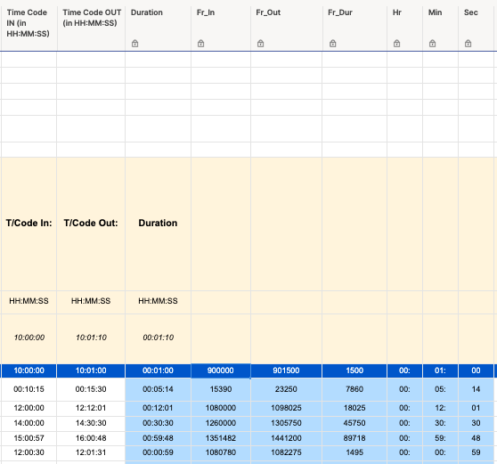
An old colleague of mine actually managed to create a sheet that was able to calculate it down to frames per second (HH:MM:SS:fps), as he was a technical whizz. The workflow is you type in the start and end times of of when an item has been shown (first 2 columns), then in column 4 (Fr_In) it uses a formula:
=IF([Time Code IN (in HH:MM:SS)]14 <> "", ((((VALUE(LEFT([Time Code IN (in HH:MM:SS)]14, 2)) * 90000)))) + (VALUE(RIGHT([Time Code IN (in HH:MM:SS)]14, 2)) + INT(VALUE(RIGHT(LEFT([Time Code IN (in HH:MM:SS)]14, 8), 2)) * 25)) + INT(VALUE(RIGHT(LEFT([Time Code IN (in HH:MM:SS)]14, 5), 2)) * 1500))
to converts the first column's value into numerics. The example on the dark blue row is, in this instance, what 10 hours equates to 900,000 frames.
An equivalent formula is then used to work out the frames per minute numerical value for the output in column 5 (Fr_Out):
=IF([Time Code OUT (in HH:MM:SS)]14 <> "", ((((VALUE(LEFT([Time Code OUT (in HH:MM:SS)]14, 2)) * 90000)))) + (VALUE(RIGHT([Time Code OUT (in HH:MM:SS)]14, 2)) * 25) + INT(VALUE(RIGHT(LEFT([Time Code OUT (in HH:MM:SS)]14, 5), 2)) * 1500))
Then the 2 figures are deducted in column 6 (Fr_Dur) to work out the difference in time duration in frames per second. My colleague then used some helper columns (the last 3 columns) to convert the value in column 6 into hours, minutes and seconds, in each associated column, using the following formulas respectively:
=IF(([Fr_Dur]14 / 90000) < 10, "0" + (INT([Fr_Dur]14 / 90000)), (INT([Fr_Dur]14 / 90000))) + ":"
=IF(INT(([Fr_Dur]14 - (INT([Fr_Dur]14 / 90000) * 90000)) / 1500) < 10, "0" + INT(([Fr_Dur]14 - (INT([Fr_Dur]14 / 90000) * 90000)) / 1500), INT(([Fr_Dur]14 - (INT([Fr_Dur]14 / 90000) * 90000)) / 1500)) + ":"
=IF(INT(([Fr_Dur]14 - (INT([Fr_Dur]14 / 1500) * 1500)) / 25) < 10, "0" + INT(([Fr_Dur]14 - (INT([Fr_Dur]14 / 1500) * 1500)) / 25), INT(([Fr_Dur]14 - (INT([Fr_Dur]14 / 1500) * 1500)) / 25))
https://us.v-cdn.net/6031209/uploads/KDN0PT3TJID0/screenshot-2021-05-14-at-17-22-57.png
I'm in the process of trying to tweak his old sheet, as for this particular use case, the team doesn't need to collate the data as granular as frames but we still need it down to the second (HH:MM:SS).
At first glance, the above might look like it's working the values out correctly but the last 2 rows, in fact, have slightly wrong duration values, by 3 and 2 seconds respectively. I appreciate this does sound pedantic, however, timings in broadcasting are essential!!
I've looked up a number of solutions in the Community Pages and then been wracking my brains trying to apply these suggestions to my problem here but I can't seem to get them to work. I'm hoping someone might be able to assist in simplifying the solution than it is currently.
I've published a version of this if it makes it any easier trying to play with the formulas: https://app.smartsheet.com/b/publish?EQBCT=b181d63d35f2473fb14c1757a0508b10. Any guidance and or pointers are much appreciated.
There are going to be a couple of key differences for you though. First, you only need to convert the time from one column instead of a start and end column. In the above solution there are always two digits for the hours, but I noticed in your example there is only one. So we need to take this formula:
=(VALUE(LEFT([Start Time]@row, 2)) * 3600) + (VALUE(MID([Start Time]@row, 4, 2)) * 60) + VALUE(RIGHT([Start Time]@row, 2))
And tweak it to this:
=(VALUE(LEFT([Start Time]@row, FIND(":", [Start Time]@row) - 1)) * 3600) + (VALUE(MID([Start Time]@row, FIND(":", [Start Time]@row) + 1, 2)) * 60) + VALUE(RIGHT([Start Time]@row, 2))
Once you have all of your times converted to numerical values, you would average this column. Then to convert it back into hh:mm:ss format, you would take the three separate columns in the linked solution of "hh:", "mm:", and "ss:" and add them all together into a single string for a single cell.
=hh: formula + mm: formula + ss: formula
-
.
@Leibel Shuchat came up with this dandy one calculating the duration between the system generated Created and Modified columns:
Title: Start Date
Formula:
=DATEONLY(Created@row)
Title: Start Time
Formula:
=IF(SUM(VALUE(LEFT(RIGHT(Created@row, LEN(Created@row) - 9), FIND(":", RIGHT(Created@row, LEN(Created@row) - 9)) - 1))) = 12, 0, SUM(VALUE(LEFT(RIGHT(Created@row, LEN(Created@row) - 9), FIND(":", RIGHT(Created@row, LEN(Created@row) - 9)) - 1)) * 60)) + SUM(VALUE(MID(Created@row, FIND(":", Created@row) + 1, 2))) + IF(RIGHT(Created@row, 2) = "PM", 720, 0) + 1
Title: End Date
Formula:
=DATEONLY(Modified@row)
Title: End Time
Formula:
=IF(SUM(VALUE(LEFT(RIGHT(Modified@row, LEN(Modified@row) - 9), FIND(":", RIGHT(Modified@row, LEN(Modified@row) - 9)) - 1))) = 12, 0, SUM(VALUE(LEFT(RIGHT(Modified@row, LEN(Modified@row) - 9), FIND(":", RIGHT(Modified@row, LEN(Modified@row) - 9)) - 1)) * 60)) + SUM(VALUE(MID(Modified@row, FIND(":", Modified@row) + 1, 2))) + IF(RIGHT(Modified@row, 2) = "PM", 720, 0) + 1
Title: Duration Minutes
Formula:
=SUM((SUM([End Date]@row - [Start Date]@row) * 24) * 60) + IF([Start Date]@row < [End Date]@row, SUM(1440 - [Start Time]@row) + [End Time]@row, [End Time]@row - [Start Time]@row)
This final column is the one that will give you the formatted days, hours, minutes:
Title: Duration
Formula:
=IF([Duration Minutes]@row > 1439, ROUNDDOWN(SUM([Duration Minutes]@row / 60) / 24, 0) + " Day" + IF(ROUNDDOWN(SUM([Duration Minutes]@row / 60) / 24, 0) > 1, "s", "") + ", ", "") + IF(MOD([Duration Minutes]@row, 1440) > 59, ROUNDDOWN(SUM(MOD([Duration Minutes]@row, 1440) / 60), 0) + " Hour" + IF(SUM(MOD([Duration Minutes]@row, 1440) / 60) > 1, "s", "") + ", ", "") + IF(MOD([Duration Minutes]@row, 60) > 0, MOD([Duration Minutes]@row, 60) + " Minute" + IF(MOD([Duration Minutes]@row, 60) > 1, "s", ""), "") + IF([Duration Minutes]@row > 0, ".", "")
.

Leibel S ✭✭✭✭✭✭
thanks for your posts about using the number stored by Smartsheet to pull the time difference. I had not heard of this before and was enlightened by the idea.
I was able to parse the information and break down how Smartsheet stores the information.
To begin:
=modified@row - Created@row will return the number of days with the decimals for the partial day.
Every day has 86,400 seconds. if you divide 1/86400 you would get 0.0000115740740740741.
However, Smartsheet only works with MAX 5 decimals which is why trying to multiply and divide the number returned by the above formula to get your time would not be accurate because it is rounded.
The way I got around this is by multiplying the number to return all the decimals not just the MAX 5 ones that show in the above formula:
=([Time Difference]@row - ROUNDDOWN([Time Difference]@row, 0)) * 100000000000000
Once we have all the full number we can then divide it by 1157407407.40741 to get the qty of seconds into the day.
You can then use the value returned from the above to return the hours, minutes, and seconds in the day:
Hours:
=INT([Total Seconds]@row / 3600) (to return the hours).
Minutes:
=INT(MOD([Total Seconds]@row, 3600) / 60)
Seconds:
=MOD([Total Seconds]@row, 60)
An example of a fully formatted column is:
="D:" + INT([Time Difference]@row) + " H:" + INT([Total Seconds]@row / 3600) + " M:" + INT(MOD([Total Seconds]@row, 3600) / 60) + " S:" + MOD([Total Seconds]@row, 60)
Please let me know if you found the above to be accurate.
Thank you
.
24 hour time to 12 hour time conversion:
=(VALUE(LEFT([Time Column]@row, FIND(":", [Time Column]@row) - 1)) - IF(VALUE(LEFT([Time Column]@row, FIND(":", [Time Column]@row) - 1))> 12, 12, 0)) + ":" + MID([Time Column]@row, FIND(":", [Time Column]@row) + 1, 2) + " " + IF(VALUE(LEFT([Time Column]@row, FIND(":", [Time Column]@row) - 1)) >= 12, "PM", "AM")
-
How would you modify this to also pull the minutes from a system-generated column?
-
@Kimberley O That is referencing a system generated column.
-
Hi Paul,
I know that I can use additional formulas and add many columns every time I want to calculate a time but it is taking time and limiting no of rows in my sheet. I really would like to have such option. Not everybody is using Smartsheet only as a project management tool and I thing Smartsheet should still look for new business opportunities.
Cheers,
Jakub
-
@Paul Newcome whoa 😵😲 this discussion thread is intense!!
Anyways, I used one of these formulas found in the thread:
=(((IF(LEFT([Th End Time]2, FIND(":", [Th End Time]2) - 1) = "12", IF(OR(FIND("a", [Th End Time]2) > 0, FIND("p", [Th End Time]2) > 0), 0, 12), VALUE(LEFT([Th End Time]2, FIND(":", [Th End Time]2) - 1))) + IF(FIND("p", [Th End Time]2) > 0, 12)) * 60 + VALUE(MID([Th End Time]2, FIND(":", [Th End Time]2) + 1, 2))) - ((IF(LEFT([Th. Time]2, FIND(":", [Th. Time]2) - 1) = "12", IF(OR(FIND("a", [Th. Time]2) > 0, FIND("p", [Th. Time]2) > 0), 0, 12), VALUE(LEFT([Th. Time]2, FIND(":", [Th. Time]2) - 1))) + IF(FIND("p", [Th. Time]2) > 0, 12)) * 60 + VALUE(MID([Th. Time]2, FIND(":", [Th. Time]2) + 1, 2)))) / 60
However if no time is entered into the Start/End times I'd like the results to return 0 to the cell. Where am I missing in this formula the 0. I'm receiving #Invalid Value when times are left blank. 🤔
Thanks
Senior Program Coordinator
De Anza College
-
@Stacey Carrasco I would just use a basic IFERROR.
=IFERROR(time_calc, 0)
-
@Paul Newcome ok sorry I'm not tracking so I should replace all my if statements with IFERROR?
Senior Program Coordinator
De Anza College
-
@Stacey Carrasco no. You would wrap the entire formula in an IFERROR. So that formula you posted before... Copy it (without the initial equals) and then paste it in my example where I have time_calc.
-
@Paul Newcome yep that was it!! 🤩👏🏆️amazing!! I was getting hung up on the paranthesis but I got it to work.
Here is the formula for reference in case anyone else needs it
=IFERROR((((IF(LEFT([W. End Time]4, FIND(":", [W. End Time]4) - 1) = "12", IF(OR(FIND("a", [W. End Time]4) > 0, FIND("p", [W. End Time]4) > 0), 0, 12), VALUE(LEFT([W. End Time]4, FIND(":", [W. End Time]4) - 1))) + IF(FIND("p", [W. End Time]4) > 0, 12)) * 60 + VALUE(MID([W. End Time]4, FIND(":", [W. End Time]4) + 1, 2))) - ((IF(LEFT([W. Time]4, FIND(":", [W. Time]4) - 1) = "12", IF(OR(FIND("a", [W. Time]4) > 0, FIND("p", [W. Time]4) > 0), 0, 12), VALUE(LEFT([W. Time]4, FIND(":", [W. Time]4) - 1))) + IF(FIND("p", [W. Time]4) > 0, 12)) * 60 + VALUE(MID([W. Time]4, FIND(":", [W. Time]4) + 1, 2)))) / 60, 0)
THANK SO MUCH!
Senior Program Coordinator
De Anza College
-
@Stacey Carrasco Glad you were able to get it sorted. 👍
-
I've tried most if not all of the formulas from this list, but not having any luck. Wondering if somehow splitting date and time from the date stamp columns causes an issue? I cannot even get it to convert to 24hrs from the first formula (to include minutes anyway).

-
@JBolan The formula you have in your screenshot is strictly for converting the hours into a 24 hour format. To get the minutes as a decimal, you will need to add a piece.
=current_formula + (VALUE(MID([Start Time]@row, FIND(":", [Start Time]@row) + 1, 2)) / 60)


