Calculating Time in HH:MM:SS

SteCoxy · 05/14/21

Hello, I'm hoping someone might be able to help me with calculating time in Smartsheet. We work with production teams in broadcasting, as well as other non-production teams, so calculating time is becoming rather vital, as more and more departments are using Smartsheet for a varying number of use cases: people and resource management, pre/post-production admin etc.

An old colleague of mine actually managed to create a sheet that was able to calculate it down to frames per second (HH:MM:SS:fps), as he was a technical whizz. The workflow is you type in the start and end times of of when an item has been shown (first 2 columns), then in column 4 (Fr_In) it uses a formula:

=IF([Time Code IN (in HH:MM:SS)]14 <> "", ((((VALUE(LEFT([Time Code IN (in HH:MM:SS)]14, 2)) * 90000)))) + (VALUE(RIGHT([Time Code IN (in HH:MM:SS)]14, 2)) + INT(VALUE(RIGHT(LEFT([Time Code IN (in HH:MM:SS)]14, 8), 2)) * 25)) + INT(VALUE(RIGHT(LEFT([Time Code IN (in HH:MM:SS)]14, 5), 2)) * 1500))

to converts the first column's value into numerics. The example on the dark blue row is, in this instance, what 10 hours equates to 900,000 frames.

An equivalent formula is then used to work out the frames per minute numerical value for the output in column 5 (Fr_Out):

=IF([Time Code OUT (in HH:MM:SS)]14 <> "", ((((VALUE(LEFT([Time Code OUT (in HH:MM:SS)]14, 2)) * 90000)))) + (VALUE(RIGHT([Time Code OUT (in HH:MM:SS)]14, 2)) * 25) + INT(VALUE(RIGHT(LEFT([Time Code OUT (in HH:MM:SS)]14, 5), 2)) * 1500))

Then the 2 figures are deducted in column 6 (Fr_Dur) to work out the difference in time duration in frames per second. My colleague then used some helper columns (the last 3 columns) to convert the value in column 6 into hours, minutes and seconds, in each associated column, using the following formulas respectively:

=IF(([Fr_Dur]14 / 90000) < 10, "0" + (INT([Fr_Dur]14 / 90000)), (INT([Fr_Dur]14 / 90000))) + ":"

=IF(INT(([Fr_Dur]14 - (INT([Fr_Dur]14 / 90000) * 90000)) / 1500) < 10, "0" + INT(([Fr_Dur]14 - (INT([Fr_Dur]14 / 90000) * 90000)) / 1500), INT(([Fr_Dur]14 - (INT([Fr_Dur]14 / 90000) * 90000)) / 1500)) + ":"

=IF(INT(([Fr_Dur]14 - (INT([Fr_Dur]14 / 1500) * 1500)) / 25) < 10, "0" + INT(([Fr_Dur]14 - (INT([Fr_Dur]14 / 1500) * 1500)) / 25), INT(([Fr_Dur]14 - (INT([Fr_Dur]14 / 1500) * 1500)) / 25))

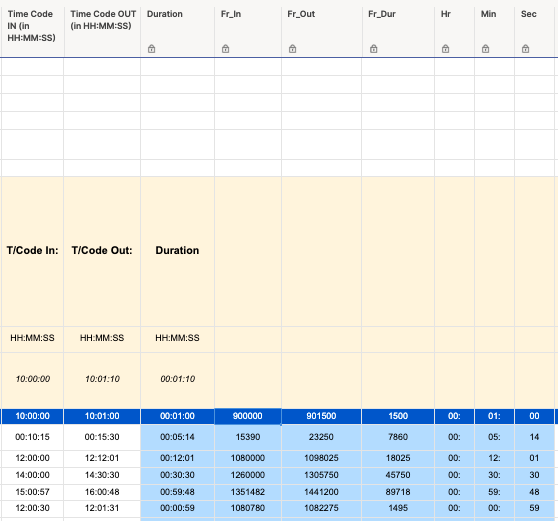
I'm in the process of trying to tweak his old sheet, as for this particular use case, the team doesn't need to collate the data as granular as frames but we still need it down to the second (HH:MM:SS).

At first glance, the above might look like it's working the values out correctly but the last 2 rows, in fact, have slightly wrong duration values, by 3 and 2 seconds respectively. I appreciate this does sound pedantic, however, timings in broadcasting are essential!!

I've looked up a number of solutions in the Community Pages and then been wracking my brains trying to apply these suggestions to my problem here but I can't seem to get them to work. I'm hoping someone might be able to assist in simplifying the solution than it is currently.

I've published a version of this if it makes it any easier trying to play with the formulas: https://app.smartsheet.com/b/publish?EQBCT=b181d63d35f2473fb14c1757a0508b10. Any guidance and or pointers are much appreciated.

Paul Newcome · 06/01/21

My apologies for the delay again. Things have been moving pretty quickly for me lately, but I am back with (hopefully) a solution.

So basically we have

Start = hh:mm:ss

End = hh:mm:ss

and you want to know the difference between the two. There are two options for the output. Going with your current layout of "hh:", "mm:", and "ss:" in their own columns, we would use something like this...

In the [Start Helper] column:

=(VALUE(LEFT([Start Time]@row, 2)) * 3600) + (VALUE(MID([Start Time]@row, 4, 2)) * 60) + VALUE(RIGHT([Start Time]@row, 2))

In The [End Helper] column:

=(VALUE(LEFT([End Time]@row, 2)) * 3600) + (VALUE(MID([End Time]@row, 4, 2)) * 60) + VALUE(RIGHT([End Time]@row, 2))

Then in the Duration column:

[End Helper]@row - [Start Helper]@row

Finally we take that total and break it out into the separate "hh:', "mm:", and "ss:" columns like so...

hh: =

=INT(Duration@row / 3600) + ":"

mm: =

=INT((Duration@row - INT(Duration@row / 3600)) / 60) + ":"

ss: =

=Duration@row - (INT(Duration@row / 3600) * 3600) - (INT((Duration@row - (INT(Duration@row / 3600) * 3600)) / 60) * 60) + ":"

Paul Newcome · 05/14/21

There is a thread (link below) that has a lot of time based solutions in it. It may take a little digging because as of right now we are up to 5 pages worth of comments and solutions. If you aren't able to find what you are looking for or need help adapting a particular solution, feel free to let me know, and I will try to help as best I can.

https://community.smartsheet.com/discussion/68947/formulas-for-calculating-time

SteCoxy · 05/14/21

Thank you @Paul Newcome. I did try looking through a number of different suggestions (including the 5 page thread) but I've ended up getting brain frazzled from a very busy week and trying to see if those suggestions could work.

I'd be most grateful if you could try and help me adapt/simplify the solution I've got - particularly to get the Fr_In, Fr_Out & Fr_Dur and Hr, Min & Sec columns' formulas simpler.

Paul Newcome · 05/14/21

Ok. I will take a look when I have more than just a few minutes to focus on it and will get back to you as soon as I can.

SteCoxy · 05/15/21

That would be much appreciated, Paul. I've published a copy of the sheet with the columns unlocked if you need access to it: https://app.smartsheet.com/b/publish?EQBCT=b181d63d35f2473fb14c1757a0508b10&_ga=2.68324883.324566985.1620639078-1939750030.1605810674

I know how the current solution works, as it's using the Time Code IN and Time Code OUT values (that are in HH:MM:SS format) to convert time into frames in the Fr_IN & Fr_OUT columns: 90000) * 90000)) / 1500). 1hr at 25 fps is 90000 frames. These 2 figures are then deducted from each other in the Fr_DUR to give you the Frame Rate Duration, which then gets converted into Hours, Minutes & Seconds in the last 3 columns, which are finally then used to convert into a HH:MM:SS format in the Duration column.

I just can't figure out how to simplify it into either Minutes IN & OUT (rather than Fr_IN & Fr_OUT) or whether those columns are even needed and if I just need the last 3 helper columns instead?

Paul Newcome · 05/17/21

My apologies for the delay. My weekend ended up being much busier than expected. I will try to take a more in depth look sometime today.

SteCoxy · 05/17/21

No need to apologise Paul - I certainly wouldn't be expecting you to look over this at the weekend. No rush required. I much appreciate your time and insight here.

SteCoxy · 05/27/21

@Paul Newcome Hi Paul, just wondering if you've had chance yet to have a look over the above?

Paul Newcome · 05/27/21

Sorry about that. Things have been rather hectic for me. I'll start taking a closer look today.

Paul Newcome · 05/27/21

So to make sure I understand...

You want to take the first two columns of time in and time out and then calculate the duration between the two.

Is there a possibility of a date overlap such as in at 11:59:00pm and out at 12:01:30am?

Will your hours always be entered as two digits such as "01" for 1am?

SteCoxy · 05/27/21

Don't worry at all Paul - you're doing me a massive favour, so no problem at all :-)

This is hopefully rather simple, in that it doesn't require date overlap - it's purely the duration of either video/audio clips that need to be calculated, rather than time in the usual sense (10am-6pm).

Paul Newcome · 05/27/21

Ok. Then the only other thing I would need to know is will the hours always be two digits such as "01" instead of "1"?

SteCoxy · 05/28/21

Yes - always 2 digits - this could be 00, 01, 11 etc.

Paul Newcome · 06/01/21