I've noticed a few people asking for Speedometer Charts in Smartsheet, so I figured I would go ahead and publish this solution that I developed. It was some years ago, so there may be better ways and / or more efficient formulas, but this should at least help get everyone started…
A few notes to kick things off…
This solution has been built so that the percentages for each of the three colors is variable.
The indicator width is also variable.
Because we had to get a bit creative, we have to use our own legend and series labels. Since we have to build our own, I figured it wouldn't hurt to get creative with these as well. We can use a section in the underlying sheet with some formulas and conditional formatting to make them more flexible.
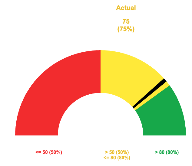
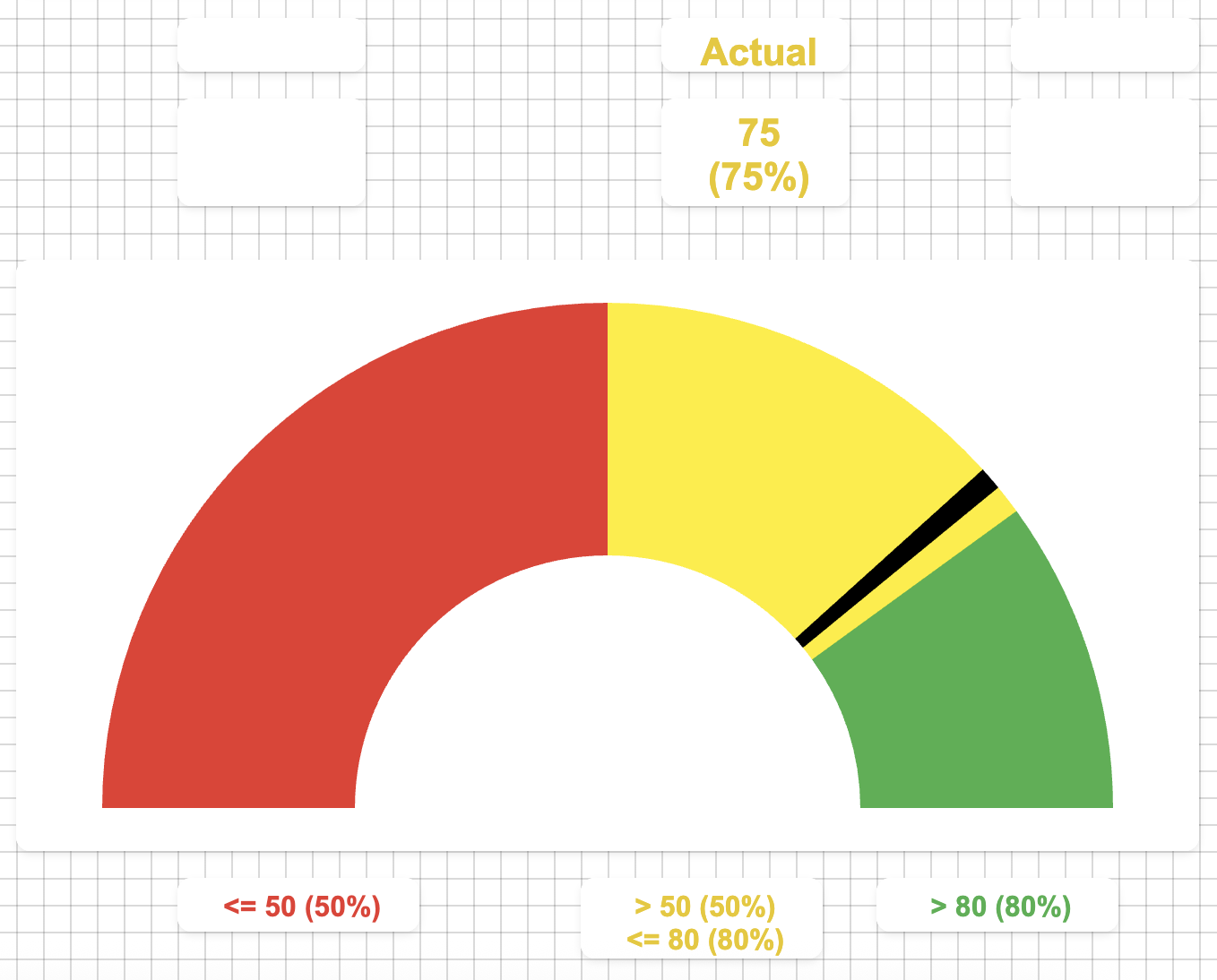
Singe the image above is static, I wanted to include that the indicator does move back and forth within the various colored sections to help visualize where within that section you really are.
This allows you to see if you are (for example) towards the lower end of yellow and in danger of going into the red or if you are in the higher end of yellow and almost into the green as opposed to just "yellow".
Basics:
There are three assets in total. A dashboard to display the chart and a sheet to format the data for the chart. These two are the focus of this thread.
The third asset will be your underlying data, but we aren't going to dive into that as there are too many different ways to collect your source data.
Below will be the details as well as screenshots for both the formatting sheet and the dashboard.
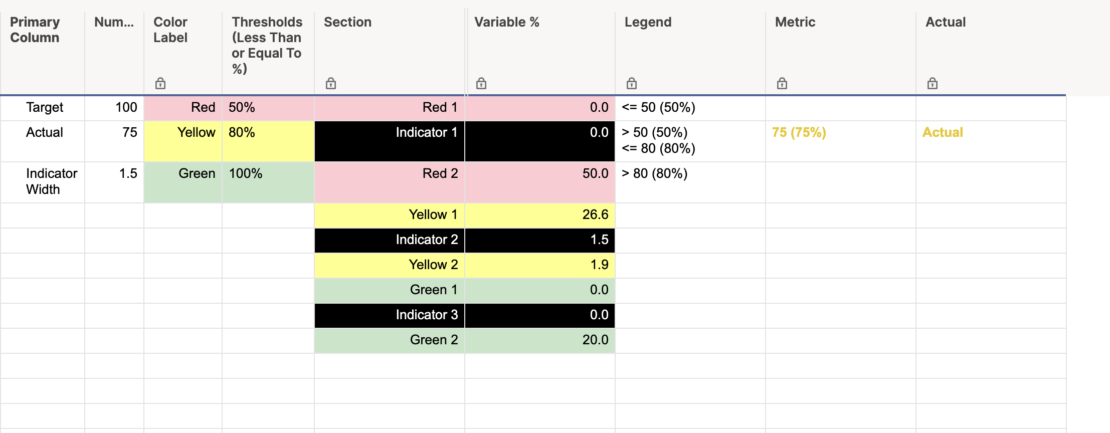
Formatting Sheet:
[Primary Column]:
NOTE: All rows in this column are manually entered.
Row 1: "Target"
Row 2: "Actual"
Row 3: "Indicator Width"
[Numbers]:
Row 1: Enter your target number. This number should be equivalent to your "100%" goal.
Row 2: This could be a cell link, a formula with a cross sheet reference, or even manually entered. This is going to be your "Actual" that is represented by the indicator in the chart.
Row 3: This is a manually entered number that indicates how wide you want the indicator in your chart. Lower numbers produce a thinner indicator, and larger numbers produce a thicker indicator. In the snippet above, the indicator width is 1.5.
[Color Label]:
NOTE: All rows in this column are manually entered.
Row 1: "Red" manually entered.
Row 2: "Yellow" manually entered.
Row 3: "Green" manually entered.
[Thresholds (Less Than or Equal To %)]:
NOTE: This column is formatted to show percentages.
Row 1: This will be the maximum percentage that would be considered "Red". For example, if you enter 50%, anything from 0% to 50% will have the indicator somewhere in the red section.
Row 2: This will be the maximum percentage that would be considered "Yellow". Using the example for Row 1, if you enter 80% here, anything above 50% but below 80% will have the indicator somewhere in the yellow section.
Row 3: 100% manually entered.
[Section]:
NOTE: All rows in this column are manually entered.
Row 1: "Red 1"
Row 2: "Indicator 1"
Row 3: "Red 2"
Row 4: "Yellow 1"
Row 5: "Indicator 2"
Row 6: "Yellow 2"
Row 7: "Green 1"
Row 8: "Indicator 3"
Row 9: "Green 2"
[Variable %]:
NOTE: All rows in this column are individual formulas.
Row 1:
=IF(Numbers2 > Numbers@row * [Thresholds (Less Than or Equal To %)]1, 0, (Numbers1 * [Thresholds (Less Than or Equal To %)]1) - ((Numbers1 * [Thresholds (Less Than or Equal To %)]1) - Numbers2) - Numbers3) + 0.00001
Row 2:
=IF(Numbers2 <= Numbers1 * [Thresholds (Less Than or Equal To %)]1, Numbers1 * (Numbers3 / 100), 0) + 0.00001
Row 3:
=IF(Numbers2 > Numbers1 * [Thresholds (Less Than or Equal To %)]1, Numbers1 * [Thresholds (Less Than or Equal To %)]1, (Numbers1 * [Thresholds (Less Than or Equal To %)]1) - Numbers2) + 0.00001
Row 4:
=IF(AND(Numbers2 < Numbers1 * [Thresholds (Less Than or Equal To %)]2, Numbers2 > Numbers1 * [Thresholds (Less Than or Equal To %)]1), (Numbers2 / (Numbers1 * [Thresholds (Less Than or Equal To %)]2)) * (Numbers1 * ([Thresholds (Less Than or Equal To %)]2 - [Thresholds (Less Than or Equal To %)]1)) - Numbers3, 0) + 0.00001
Row 5:
=IF(AND(Numbers2 <= Numbers1 * [Thresholds (Less Than or Equal To %)]2, Numbers2 > Numbers1 * [Thresholds (Less Than or Equal To %)]1), Numbers1 * (Numbers3 / 100), 0) + 0.00001
Row 6:
=IF(AND(Numbers2 < Numbers1 * [Thresholds (Less Than or Equal To %)]2, Numbers2 > Numbers1 * [Thresholds (Less Than or Equal To %)]1), (Numbers1 * ([Thresholds (Less Than or Equal To %)]2 - [Thresholds (Less Than or Equal To %)]1)) - ((Numbers2 / (Numbers1 * [Thresholds (Less Than or Equal To %)]2)) * (Numbers1 * ([Thresholds (Less Than or Equal To %)]2 - [Thresholds (Less Than or Equal To %)]1))), Numbers1 * ([Thresholds (Less Than or Equal To %)]2 - [Thresholds (Less Than or Equal To %)]1)) + 0.00001
Row 7:
=IF(Numbers2 > Numbers1 * [Thresholds (Less Than or Equal To %)]2, MIN((Numbers1 * ([Thresholds (Less Than or Equal To %)]3 - [Thresholds (Less Than or Equal To %)]2)) - (Numbers1 - Numbers2), Numbers1) - Numbers3, 0) + 0.00001
Row 8:
=IF(Numbers2 > Numbers1 * [Thresholds (Less Than or Equal To %)]2, Numbers1 * (Numbers3 / 100), 0) + 0.00001
Row 9:
=IF(Numbers2 >= Numbers1, 0, IF(Numbers2 > Numbers1 * [Thresholds (Less Than or Equal To %)]2, (Numbers1 * ([Thresholds (Less Than or Equal To %)]3 - [Thresholds (Less Than or Equal To %)]2)) - ((Numbers1 * ([Thresholds (Less Than or Equal To %)]3 - [Thresholds (Less Than or Equal To %)]2)) - (Numbers1 - Numbers2)), Numbers1 - (Numbers1 * [Thresholds (Less Than or Equal To %)]2))) + 0.00001
[Legend]:
NOTE: All rows in this column are individual formulas.
Row 1:
="<= " + ROUND((Numbers1 * [Thresholds (Less Than or Equal To %)]@row)) + " (" + ROUND([Thresholds (Less Than or Equal To %)]@row * 100) + "%)"
Row 2:
="> " + ROUND(Numbers1 * [Thresholds (Less Than or Equal To %)]1) + " (" + ROUND([Thresholds (Less Than or Equal To %)]1 * 100) + "%)" + CHAR(10) + "<= " + ROUND((Numbers1 * [Thresholds (Less Than or Equal To %)]2)) + " (" + ROUND([Thresholds (Less Than or Equal To %)]@row * 100) + "%)"
Row 3:
="> " + ROUND((Numbers1 * [Thresholds (Less Than or Equal To %)]2)) + " (" + ROUND([Thresholds (Less Than or Equal To %)]2 * 100) + "%)"
[Metric]:
NOTE: All rows in this column are individual formulas.
Row 1:
=IF(Numbers2 <= Numbers1 * [Thresholds (Less Than or Equal To %)]1, Numbers2 + " (" + ROUND(Numbers2 / Numbers1, 2) * 100 + "%)", 0)
Row 2:
=IF(AND(Numbers2 > Numbers1 * [Thresholds (Less Than or Equal To %)]1, Numbers2 <= Numbers1 * [Thresholds (Less Than or Equal To %)]2), Numbers2 + " (" + ROUND(Numbers2 / Numbers1, 2) * 100 + "%)", 0)
Row 3:
=IF(Numbers2 > Numbers1 * [Thresholds (Less Than or Equal To %)]2, Numbers2 + " (" + ROUND(Numbers2 / Numbers1, 2) * 100 + "%)", 0)
[Actual]:
NOTE: All rows in this column are manually entered.
Row 1, Row 2, and Row 3 all have the word "Actual" anually entered.
Conditional Formatting:
NOTE: I wasn't able to show it in the screenshot, but each rule is applied to the [Metric] and [Actual] columns.
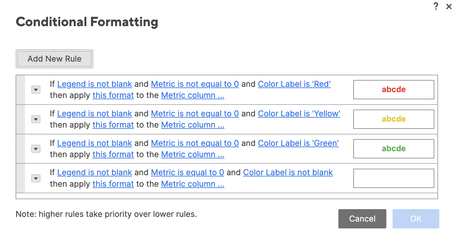
Screenshot of the formatting sheet:
Dashboard:
You can use your own judgement for the sizes of each widget, but the general idea here is that we use individual metrics widgets to display the actuals and the "legend", and we use a half-donut chart for the "speedometer" portion.
You can see in the below screenshot how each of the widgets are laid out. I have the "Actuals" going across the top relatively in line with each of their colored sections, and the legend is metrics widgets across the bottom also in line with each of the colored sections.
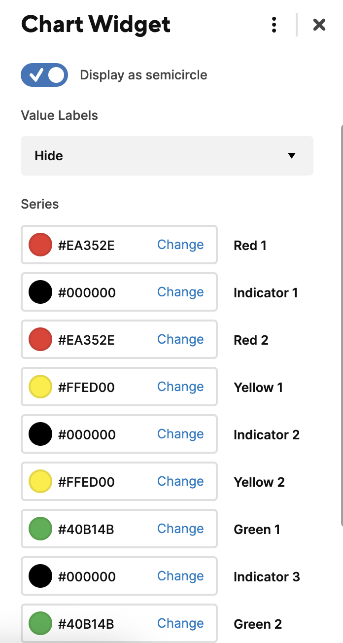
The "star of the show" here though is the speedometer chart. When we select the data for this, we select rows 1 through 9 of both the [Section] column and the [Variable %] column. I will provide a separate snippet of the chart series to show what colors were selected for the above.
Widget Layout:
Series: