Best Of

Hi @Marcela Hernandez

You can use the value of Sheet A to be prefilled in the form of Sheet B, whose form URL or Link is placed in Sheet A using a technique called "URL query string." Then, you can refer to the form input value in Sheet B from Sheet A.

https://help.smartsheet.com/articles/2478871-url-query-string-form-default-values

https://app.smartsheet.com/b/publish?EQBCT=ece05f810a2d4f3887960b6a538a382e

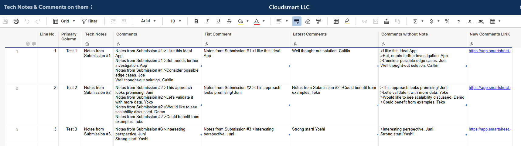
In the above sheet, if you click one of the links at the far left, you will see a form like this.

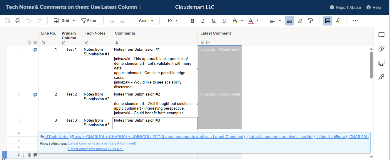
Please note that the form user can edit the New Comments' "Notes from Submission #1 >" as the row No.3's last comment shows.

So, is the [Line No.] value 1.

Therefore, the form below is for illustrative purposes, but in actual use, you should hide the Line No. field because changing the number would cause the input to go to the wrong place.

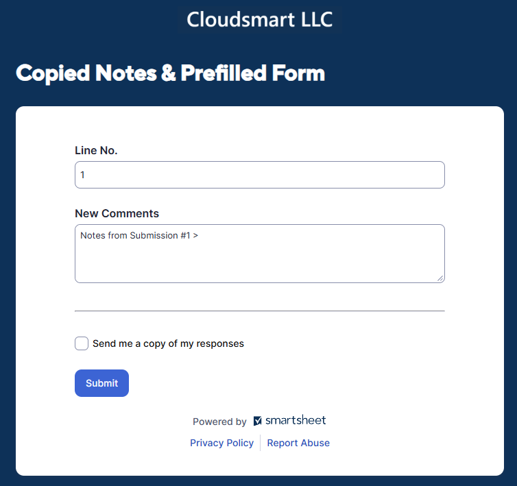
The values like 1 or 'Notes from Submission #1 >' are prepopulated by this formula;

[New Comments LINK] =[Form URL]# + SUBSTITUTE(SUBSTITUTE(SUBSTITUTE("?Line No.=" + [Line No.]@row + "&New Comments=" + [Tech Notes]@row + " > ", " ", "%20"), "#", "%23"), ">", "%3E")

The SUBSTITUTE function is used to replace special characters like space, "#", or ">" with ones that are not affected in the link. Please look at the help article at the top for details.

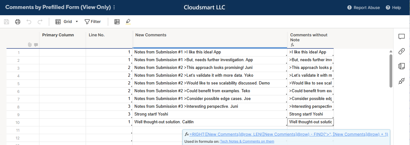
The form inputs the data to Sheet B;

https://app.smartsheet.com/b/publish?EQBCT=43f5ba7a4955460480760ac30968ccb8

Then, you can reference them in Sheet A with formulas like these using the [Line No.] as a key.

[Comments] =JOIN(COLLECT({Comments by Prefilled Form : New Comments}, {Comments by Prefilled Form : Line No.}, [Line No.]@row ), CHAR(10))

[Fist Comment] =IFERROR(INDEX(COLLECT({Comments by Prefilled Form : New Comments}, {Comments by Prefilled Form : Line No.}, [Line No.]@row ), 1), "")

[Latest Comments] =IFERROR(INDEX(COLLECT({Comments by Prefilled Form : New Comments}, {Comments by Prefilled Form : Line No.}, [Line No.]@row ), COUNTIF({Comments by Prefilled Form : Line No.}, [Line No.]@row )), "")

[Comments without Note] =JOIN(COLLECT({Comments by Prefilled Form : Comments w/o Notes}, {Comments by Prefilled Form : Line No.}, [Line No.]@row ), CHAR(10))

@Marcela Hernandez

Method 1: Hide Columns

In this method, I hide all the unwanted columns and change the 'Comments without Note' column to add one Tech Note at the top, as shown in the 'One note and Comments' column.

https://app.smartsheet.com/b/publish?EQBCT=7fa790e49ea441fe932e8a9be0b9f92b

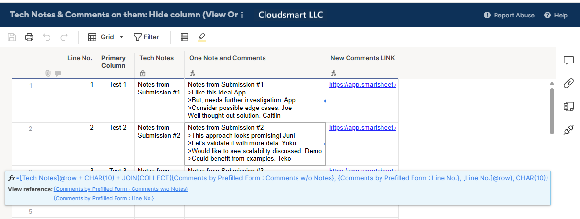
=[Tech Notes]@row + CHAR(10) + JOIN(COLLECT({Comments by Prefilled Form : Comments w/o Notes}, {Comments by Prefilled Form : Line No.}, [Line No.]@row ), CHAR(10))

This method is good if your commentator has viewer access to the sheet, and can not add comments to rows or the sheet.

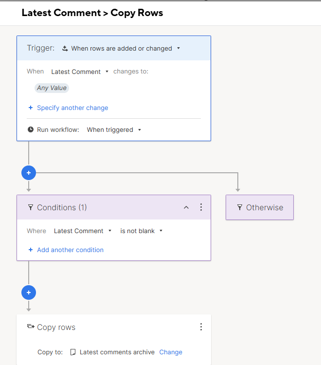
Method 2: Latest Comment Special Column + Copy rows automation

If your commentator has commenter or editor access, you can use the Latest Comment special column.

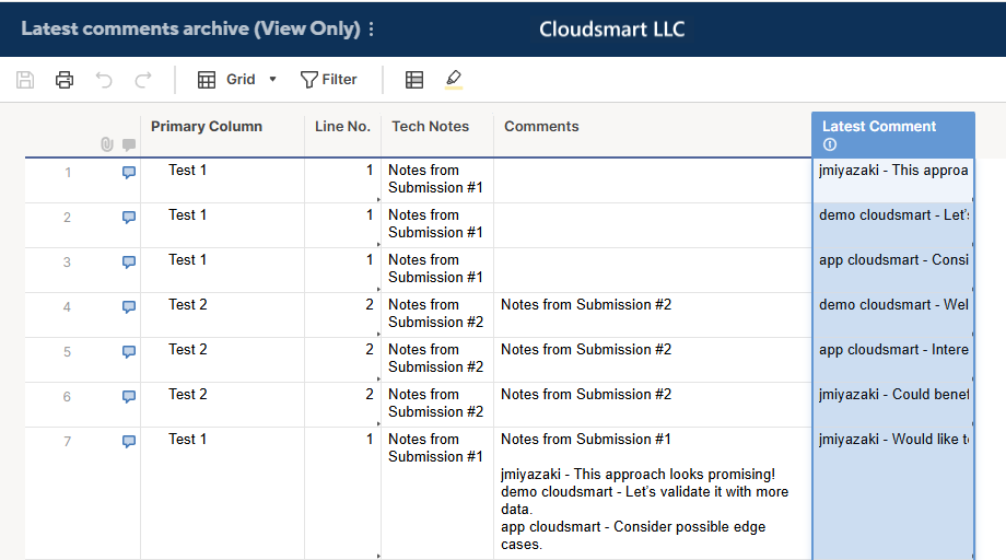
The latest row comment will automatically populate the column, and with automation, you can copy the row to another sheet. Then, using Line No. as a key, you can refer to those comments.

https://app.smartsheet.com/b/publish?EQBCT=c0b3a52d580043abbd61c81223e47fb1

https://app.smartsheet.com/b/publish?EQBCT=aec11f18e0bf450d9fa87b32d7786084

I have a couple of comments on this topic for your reference, if you are interested in this method.

Is there a way to collect all comments in one cell?

Moving Comments Between Sheets

Central Location for User Comments across Smartsheet

@k_Hunter001 Smartsheet can't perform that type of validation in a grid view. The only view in Smartsheet that could do that type of validation would be Dynamic View.

Otherwise, you'd have to use another 3rd party form solution that can enforce that type of logic.

Hi @RiseUpPNW

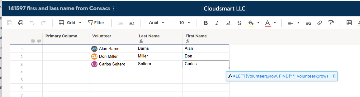
You need to change the First Name's formula to this;

=LEFT(Volunteer@row , FIND(" ", Volunteer@row ) - 1)

In English, find the space between the first name and last name. Get the string from the top up to position one before the found space position to get the first name.

https://app.smartsheet.com/b/publish?EQBCT=e1858249b1eb43d08b95fe92860b5cd5

I would insert a helper column that outputs the level

=COUNT(ANCESTORS())

Then you can leverage this in whatever other formula you are using to evaluate the levels.

=COUNTIFS(………………….., Level:Level, @cell = 2)

Hey Brandon, would this do the trick?

=SUMIFS({Upcoming Jobs (High Level) Range 3}, {Upcoming Jobs (High Level) Range 1}, OR(@cell = [Job Name 1]@row , @cell = [Job Name 2]@row , @cell = [Job Name 3]@row , @cell = [Job Name 4]@row ))