Multiple IF / AND / OR Statements Help, Please.

AHottman

This is such a great community and a wealth of knowledge for a new Smartsheet user like me. I have done several formulas, but this one has me scratching my head. 

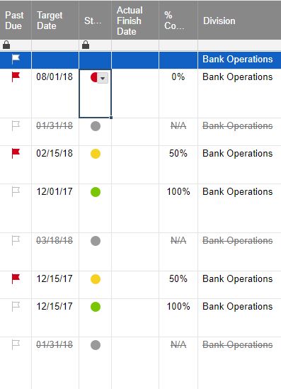
I have a [Target Date] column, [% Complete] column, and status column that I would like to automate with Red, Yellow, Green, and Gray status balls. The [% Complete] column is a drop-down with options: N/A, 0%, 25%, 50%, 75%, and 100%. 

I would like to have no status ball for "N/A". That seems to be the easy part.

Next, I would like the status ball to be Gray if the [% Complete] is 0% and the target date is 5+ days out and Green if the [% Complete] is 25%, 50%, or 75% and 5+ days out. I would like the status balls to change to Yellow if the [% Complete] is 0%, 25%, 50%, or 75% and 3 days or less from [Target Date], and have status balls change to Red if the [% Complete] is 0%, 25%, 50%, or 75% and the [Target Date] is the date before the target date, date of target date, or is past the target date. 

I won't need a status ball for [% Complete] = 100%, as I plan to set conditional formatting to show a completed task. 

I've tried several different variations today and am getting two different formula error messages. I thought I'd post this question, as there are several of you experienced users who seem to excel at these formulas. 

Thank you in advance for your assistance! 

Mike Wilday

Any chance you could show us what you created so we can walk you through what to shift to make your formulas work? 

You are going to have to nest several if statements with And statements to make this happen. 

 

AHottman

Thank you very much for your reply and offer to assist me in this undertaking. I have attached a small sample of a very large task list. The status balls are currently set to be gray if N/A, red if 0% complete, green if in progress or 100%. The risk flags are on/off for tasks that are not 100% complete and past due. In rethinking the status balls, we'd really prefer to have them as I've indicated above and use the conditional formatting and filters to de-clutter the N/A and 100% complete tasks. Thanks again for offering to assist; it is appreciated. 

Javed Hassan

Plug this into the first row and copy the formula down and it should work. I added a part at the beginning that says if the Target date is blank, then the symbol should be blank. It's the first IF formula, so just replace that second "" with a color if needed.

=IF([Target Date]1 = "", "", (IF([% Complete]1 = 1, "", IF(AND([% Complete]1 = 0, [Target Date]1 >= TODAY() + 5), "Gray", IF(AND([% Complete]1 < 1, [Target Date]1 >= TODAY() + 5), "Green", IF(AND([% Complete]1 < 1, [Target Date]1 <= TODAY()), "Red", "Yellow"))))))

J. Craig Williams

A few comments on the solution from the Peanut Gallery:

As new users, try to get into the habit of using @row instead of the current row number for references to cells on the same row. It will save you a few headaches in the future when copying things around. It will also aid the transition to a column default formula if Smartsheet ever releases that feature.

Second, TODAY()+5 and TODAY(5) are functionally equivalent. I find the second easier to read and less likely to have errors.

I also removed one unnecessary () pair.

The new formula would look like this:

=IF([Target Date]@row = "", "",

 IF([% Complete]@row = 1, "",

 IF(AND([% Complete]@row = 0,[Target Date]@row >= TODAY(5)), "Gray",

 IF(AND([% Complete]@row < 1, [Target Date]@row >= TODAY(5)), "Green",

 IF(AND([% Complete]@row < 1, [Target Date]@row <= TODAY()), "Red",

 "Yellow")))))

Personally, I have a few places where I turn off conditional formatting temporarily, so I tend to avoid blanks when the cell value has meaning, but not importance in most cases. I point that out primarily for anyone looking here for the most recent answer and assuming it will fix their own problem. I would need to further modify it for my own solution because there is a still a piece missing (the formatting).

Lastly, I prefer to avoid duplication of criteria when using Nested IF's, so I would rewrite the formula as so:

=IF([Target Date]@row = "", "", IF([% Complete]@row = 1, "", IF([Target Date]@row >= TODAY(5), IF([% Complete]@row = 0, "Gray", "Green"), IF(AND([% Complete]@row < 1, [Target Date]@row <= TODAY()), "Red", "Yellow"))))

This results in a formula that is shorter (less processing needed) and easier to maintain, in my opinion.

=IF([Target Date]@row = "", "",

 IF([% Complete]@row = 1, "",

 IF([Target Date]@row >= TODAY(5), 

   IF([% Complete]@row = 0, "Gray", "Green"),

 IF(AND([% Complete]@row < 1, [Target Date]@row <= TODAY()), "Red",

 "Yellow"))))

Craig

AHottman

Thank you! I really appreciate the help! 

AHottman

Craig - 

Thank you very much for the help with the formula and additional helpful advice. I appreciate you taking the time and your willingness to help those of us just getting started with Smartsheet. I appreciate and enjoy learning, and you have taught me something. 

Thanks again, Amy 

J. Craig Williams

Then my work here is done Amy.

Craig

nmitchell

Hello, I have a similar situation where I'm trying to use multiple IF(OR statements to determine risk status based on six different factors. So, if any of the factors are "High" then the output is "High", if false, then if any of the factors are "medium" then the output is "Medium", if false, then if any of the factors are "Low" then the output is "Low". There is actually potential that I would need to add a fourth status which would be "Not Approved" which would be first scenario (but I think I can figure out how to add that if I can get the rest of it correct first).

What I have done is this but I'm getting "INCORRECT ARGUMENT" or "High" for every line:

=IF(OR([Early Procurement Risk]@row = "High", [Vendor Prepayment Risk]@row = "High", [SLA Penalties Risk]@row = "High", [Parent Guarantee Risk]@row = "High", [Fixed Labor Rates Risk]@row = "High", [Liquidated Damages Risk]@row = "High"),

"High",

IF(OR([Early Procurement Risk]@row = "Medium", [Vendor Prepayment Risk]@row = "Medium", [SLA Penalties Risk]@row = "Medium", [Parent Guarantee Risk]@row = "Medium", [Fixed Labor Rates Risk]@row = "Medium", [Liquidated Damages Risk]@row = "Medium",

"Medium",

IF(OR([Early Procurement Risk]@row = "Low", [Vendor Prepayment Risk]@row = "Low", [SLA Penalties Risk]@row = "Low", [Parent Guarantee Risk]@row = "Low", [Fixed Labor Rates Risk]@row = "Low", [Liquidated Damages Risk]@row = "Low"),

"Low", "N/A"))))

Anyone that can help with this?

nmitchell

After continuing to mess with this, I found there was a ")" missing after the "Medium" OR statement. I also updated to include the first condition of "Not Approved" and everything appears to be working:

=IF([Fixed Labor Rates Risk]@row = "Not Approved", "Not Approved",

IF(OR([Early Procurement Risk]@row = "High", [Vendor Prepayment Risk]@row = "High", [SLA Penalties Risk]@row = "High", [Parent Guarantee Risk]@row = "High", [Fixed Labor Rates Risk]@row = "High", [Liquidated Damages Risk]@row = "High"), "High",

IF(OR([Early Procurement Risk]@row = "Medium", [Vendor Prepayment Risk]@row = "Medium", [SLA Penalties Risk]@row = "Medium", [Parent Guarantee Risk]@row = "Medium", [Fixed Labor Rates Risk]@row = "Medium", [Liquidated Damages Risk]@row = "Medium"), "Medium",

IF(OR([Early Procurement Risk]@row = "Low", [Vendor Prepayment Risk]@row = "Low", [SLA Penalties Risk]@row = "Low", [Parent Guarantee Risk]@row = "Low", [Fixed Labor Rates Risk]@row = "Low", [Liquidated Damages Risk]@row = "Low"), "Low",

"N/A"))))

Kavish

Hello, hope you are having a great day, I have a similar issue using IF/AND combinations in formulae. I am trying to get a status off the percentage calculated in a different field (percentage value) and keep getting this error that says - #INCORRECT ARGUMENT SET

This is my Formula- Details8 is the field where the percentage is calculated

=IF(Details8 = 0, "Not Started", IF(AND(Details8 >= 0.01, Details8 <= 0.59), "Below Expectations"), IF(AND(Details8 >= 0.6, Details8 <= 0.7), "Needs Improvement"), IF(AND(Details8 >= 0.8, Details8 <= 0.94), "Meeting Expectations"), IF(AND(Details8 >= 0.95, "Exceeding Expectations")))

Any and all assistance here would be appreciated. Thank you in advance!

heyjay

https://community.smartsheet.com/discussion/comment/447106#Comment_447106

@Kavish

=IF(Details@row = 0, "Not Started",
IF(AND(Details@row >= 0.01, Details@row <= 0.59), "Below Expectations",
IF(AND(Details@row >= 0.6, Details@row <= 0.7), "Needs Improvement",
IF(AND(Details@row >= 0.8, Details@row <= 0.94), "Meeting Expectations",
IF(Details@row >= 0.95, "Exceeding Expectations", "")))))

BTW you are missing >= 0.71 and < = 0.79