Formula for text columns convert to sum?

Hello,
I'm trying to help build a sort of prioritization scorecard into a sheet. We have 4 columns, each with possible values of (example) "A", "B" or "C", and would like to have another column that sums each based on assigning a number value to each dropdown option.
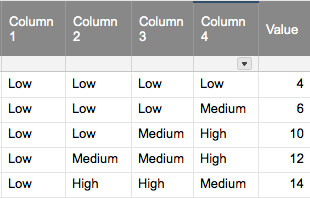
So for example, the columns and their possible dropdowns:
Column 1 - A, B, C
Column 2 - A, B, C
Column 3 - A, B, C
Column 4 - A, B, C
Where A = 1, B = 2, C = 3
IF Column 1 = A, Column 2 = B, Column 3 = A, and Column 4 = C, the total value presented would be 7 (1 + 2 + 1 + 3).
I'm aware we could add 4 additional columns to present the numerical value attached to each, then a 5th column with the sum of those. However, I'll be frank: this is a monster sheet and adding even more columns when I'm hoping for a "simple" formula makes me want to cry.
Any suggestions? From what I'm reading on other forum posts I *think* this is impossible but would really appreciate a confirmation. Thanks!
Comments
Are the 4 columns adjacent? You could add multiple COUNTIF statements together:
=COUNTIF([Column 1]@row:[Column 4]@row, "A") + (COUNTIF([Column 1]@row:[Column 4]@row, "B") * 2) + (COUNTIF([Column 1]@row:[Column 4]@row, "C") * 3)
I suppose the columns wouldn’t even need to be adjacent as long as the columns in between don’t contain just A,B, or C.
Hi Brian, thanks for your help but I'm thinking we crossed wires somewhere.
Let me flesh out the information a bit. So here's what the columns are actually representing:
Scorecard criteria 1:
- Low
- Medium
- High
Scorecard criteria 2:
- Low
- Medium
- High
Scorecard criteria 3:
- Low
- Medium
- High
Scorecard criteria 4:
- Low
- Medium
- High
For all columns:
- Low = 1
- Medium = 3
- High = 5
So, as an example of a real-world use:
Scorecard criteria 1: Low (((1)))
Scorecard criteria 2: High (((5)))
Scorecard criteria 3: High (((5)))
Scorecard criteria 4: Medium (((3)))
The formula in a fifth column would return a total of "14" (since there was one "Low", two "High"s, and one "Medium").
Does that make more sense?
It sounds like this formula should work for you, unless there’s something I’m missing:
=COUNTIF([Column 1]@row:[Column 4]@row, "Low") + (COUNTIF([Column 1]@row:[Column 4]@row, "Medium") * 3) + (COUNTIF([Column 1]@row:[Column 4]@row, "High") * 5)
This formula assumes that your criteria columns are named Column 1, Column 2, Column 3, and Column 4. The formula searches all the cells in a row between Column 1 and Column 4 and counts the instances of Low, Medium, High, then multiplies those counts by 1, 3, and 5 respectively and adds them together.
Way to go Brian!! That's exactly what we were looking for. Thank you so much for your help, much appreciated!!
Sorry Brian, in my excitement at your perfect answer I forgot to ask one more add-on. This isn't something we're implementing on Day 1 so it's okay if we can't figure it out right now. But after the countif, is there a way of populating (instead of the numerical value) a word? So, for example, if the overall score comes back as between 0 and 10, the value shown in the cell should be something like "Low importance". If it's between 10-20, it should read "Medium importance", etc. What's the framework for adding something like that if at all? Many thanks again.
Sure. You could use the formula in a nested IF formula:
=IF(COUNTIF([Column 1]@row:[Column 4]@row, "Low") + (COUNTIF([Column 1]@row:[Column 4]@row, "Medium") * 3) + (COUNTIF([Column 1]@row:[Column 4]@row, "High") * 5) >= 20, "High Importance", IF(COUNTIF([Column 1]@row:[Column 4]@row, "Low") + (COUNTIF([Column 1]@row:[Column 4]@row, "Medium") * 3) + (COUNTIF([Column 1]@row:[Column 4]@row, "High") * 5) >= 10, "Medium Importance", IF(COUNTIF([Column 1]@row:[Column 4]@row, "Low") + (COUNTIF([Column 1]@row:[Column 4]@row, "Medium") * 3) + (COUNTIF([Column 1]@row:[Column 4]@row, "High") * 5) > 0, "Low Importance")))
In this version, it returns “High Importance” if the count is 20+, "Medium Importance” if 10-19, or "Low Importance” for 1-9.