Please help with a formula!

belliott76966

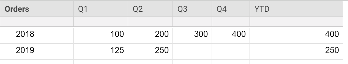
I am looking to compare Year to Date numbers, and I'm having a hard time figuring out a formula to do so. I've attached a sample screen shot. At the end of the day, I'm trying to add a metric into a dashboard that shows 2018 vs 2019 year to date. I created the "YTD" column that shows the value of the last column that has data in it on the right side of the row, which works great for the current year. But for 2018, I need to somehow calculate tell it to "Look at the last row with data (other than YTD) and deliver the number above that". Does that make sense? Any way I can do that? I know it looks like I could easily type it in once per quarter, but I'm using this as an example. We are actually doing weekly tracking.

Thanks in advance!

~Bill

Mike Wilday

I'd put YTD right after the order column. Then you can put the comparison on the dashboard fairly easily... 

https://www.screencast.com/t/8Pfo3qgd

belliott76966

Hi Mike,

Thanks for taking the time to do that! I don't think it will quite do the trick... what I need it to do is pull the 200 number in my original example to compare against the 250. The problem is that the YTD column pulls the final 400 number. 

Nic Larsen

I suppose if you swapped the column headers for years and ran the quarters down the vertical. You could use a MAX formula to review the column range and pull the max number out and feed that to your dashboard. Or do this through a roll up sheet if your source sheet needs to keep its format. 

Paul Newcome

Put this in the YTD column in the 2018 row and see how it works for you (I am assuming 2018 is on row 1)...

 

=INDEX([Q1]1:[Q4]1, 1, COUNTIFS([Q1]2:[Q4]2, ISNUMBER(@cell)))

 

Basically you are using an INDEX function to pull data from a range based on row and column requirements. If you set the range as across a row ([Q1]1:[Q4]1), then naturally the row index would be 1. To then determine the column index, we will first look at the row below it that you are wanting to compare to ([Q1]2:[Q4]2) and count how many of the cells in that range contain a number. That count will give you your column index.

 

So basically this formula is saying to look at the data from the first range with the row being 1 (naturally since the range is only one row anyway) and then pull the data from the # column and basing the # on how many are filled in below it.

belliott76966

This worked beautifully, thank you!