SUMIF Formula

refogleman91066

Working on a project where I want to put a total in a column based on if an asset needs a rehab.  I would like for the formula to find the year and if it matches with the column, put the total in that cell. 

Here's what I've got:

=SUMIF([Next Overhaul Year]2:[Overhaul 15]2, =[SFY2021]1, [Dry Dock Cost]@row)

Getting an invalid argument set error message.  

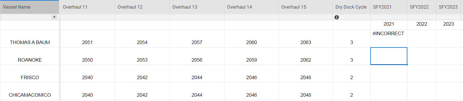
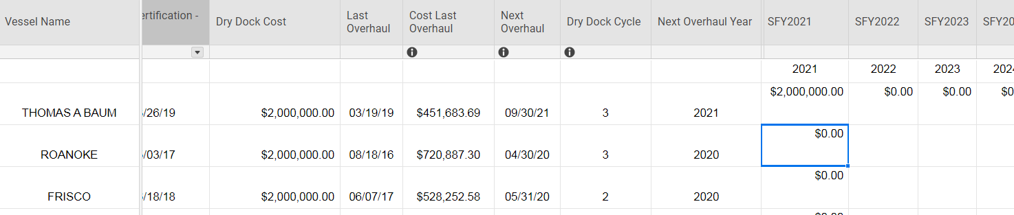
Here's a screen shot for reference:

L_123

https://help.smartsheet.com/function/sumif

---------------------------------------------------------------------------------

=SUMIF(range, criterion,[sum_range])

Range: The range to analyze

Criterion: The criteria for said range

[sum_range]: in hard brackets because it is optional. If included, this will be the range summed up. otherwise, first range will be summed.

*(The number of cells in both ranges must be equal to each other)

----------------------------------------------------------------------------------

Beyond that, I cannot write your formula as I don't understand how you are associating the date with the values.

refogleman91066

I'm trying to put a value in a cell if any of those years in that range equals the year in the column. Does that help?

refogleman91066

So the sum range is where I'm going wrong.  The "range" for me is just a single cell.  So, I regrouped and tried this formula:

=IFERROR(IF(MATCH(2021, [Next Overhaul Year]@row:[Overhaul 15]@row), [Dry Dock Cost]@row, 0), 0)

It works for the first cell, but when I drag it down, it's not working properly. 

Paul Newcome

Try using a CONTAINS function within an IF statement.

 

=IF(CONTAINS(2021, [Next Overhaul Year]@row:[Overhaul 15]@row), [Dry Dock Cost]@row)

refogleman91066

That didn't work either.  Lemme try a different approach and post below.

refogleman91066

I'm trying to budget out how much it will cost to pay for dry docks for each boat each year.  The cost is set and I have the date for the next scheduled dry dock and each boat is on a 2, 3, or 5 year cycle, depending on the boat. Is there a way to project out by year based on the dry dock cycle? I started with this formula:

=SUMIF([Next Overhaul Year]2, [SFY2021]$1, [Dry Dock Cost]@row)

So, I want to calculate for 2022 - 2050.  Screenshot below for reference.

L_123

=SUMIF([Next Overhaul Year]:[Next Overhaul Year], 2021, [Dry Dock Cost]:[Dry Dock Cost])

This will work for 2021, but it will be a pain to drag it, as you will have to type it in every time. Also you will have a long list of historical projections I would imagine are rather useless. I would name the columns you currently have posted as the year as 1-30 or something similar so it isn't confusing when the years don't match up, then use this formula in the first row:

=year(today())+1

Then post the expected results in the second row as the formula

=SUMIF([Next Overhaul Year]:[Next Overhaul Year], year(today())+count([1]$1:[1]1), [Dry Dock Cost]:[Dry Dock Cost])

or something similar. This way you can drag the formula easily, and it will always show the next 30 years.