How do you apply the same conditional formating to multiple cells?

Sean O'Brien

In excel I can create a formula in a cell, then create conditional formatting on that cell. For example, I can do a quick formula to compare to values. If the value is <0 apply a format that makes the cell red.

I can then cut and paste that cell into any other cell I want in a spreadsheet and it gets the formula and the conditional formatting.

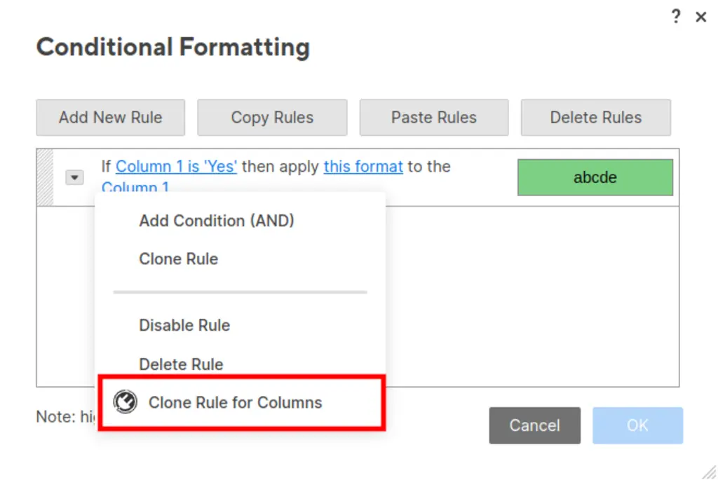
I've attached a screen shot showing a smartsheet and the cells that would be shaded red in this example.

This spreadsheet has about 25 columns that need this rule applied to them, and each column has a dozen rows that have the need to be shaded.

How can this be accomplished in Smartsheet?

Paul Newcome

@lewis hamilton Your post is again referencing Excel and will not work in Smartsheet.

@Sean O'Brien If you only want it to apply to specific rows, then you will need to add in a condition to the rule that will locate something unique to the row(s) you want the formatting to apply to such as specific text in another column that is unique to those particular rows or even creating a checkbox column, checking the box for those particular rows, then building that criteria into your Conditional Formatting rule.

Additionally you are correct that you will need a separate rule for each column to be evaluated individually.

Jennifer Whitlock

Smartsheet has a Conditional Formatting button on the top toolbar:

If you use that function, you should be able to create rules of formatting for any number of cells or columns. You can select the range, criteria, and where to apply the formatting. That should solve your issues without a need for formulas.

Hope this helps!

Sean O'Brien

I've tried that without success. I cannot find a way to apply the rule to the CELLS I want, not the columns or rows.

I don't want to change more than one cell based upon one condition. I want each cell to be evaluated based upon the same condition (contents<0) and then have the color for that one cell changed.

I should note that the formula has nothing to do with this issue, it just happens to be the cells I want to format also have formula in them. I can cut and paste the formula into other cells in the smartsheet without issue, but the conditional formatting doesn't transfer with the cut and paste.

Jennifer Whitlock

Hi again Sean,

If the criteria you're trying to set is, for example, that there is less than 0 Virtual Servers, you would open the conditional formatting box, select "Add New Rule" and set something like:

<set condition> = Servers - Virtual is less than 0

this format = highlighted in red

and change entire row to just the column containing the cells that should be highlighted.

You can then copy that rule and change the columns to include any other conditions you want to match.

Hopefully these screenshots help as well.

Sean O'Brien

Well, I'm certain I did exactly this and it didn't work as expected but I will try it again.

So if I'm reading this correctly if I have 30 columns I'll need 30 rules?

Sean O'Brien

-

Sean O'Brien

And this seems to apply it to every single cell in the column, so ANY cell that is <0 gets formatted, not just the total row that I want.

Jennifer Whitlock

Hi Sean,

If you want to add a condition to a rule, so that only the rows that you have shaded in dark purple in your screenshot will be formatted vs. all of the cells in a column, you can add a condition by clicking the drop down to the left of the rule.

This is the only method of conditional formatting that I am familiar with in Smartsheet. I'm sorry if I haven't been able to help solve this for you.

Sean O'Brien

Am I right in thinking I'll need a rule for every column I want this to apply to?

Paul Newcome

@lewis hamilton Your post is again referencing Excel and will not work in Smartsheet.

@Sean O'Brien If you only want it to apply to specific rows, then you will need to add in a condition to the rule that will locate something unique to the row(s) you want the formatting to apply to such as specific text in another column that is unique to those particular rows or even creating a checkbox column, checking the box for those particular rows, then building that criteria into your Conditional Formatting rule.

Additionally you are correct that you will need a separate rule for each column to be evaluated individually.