Is there a way to highlight values by month or display values by month in a gnatt view?

mbsamuel6

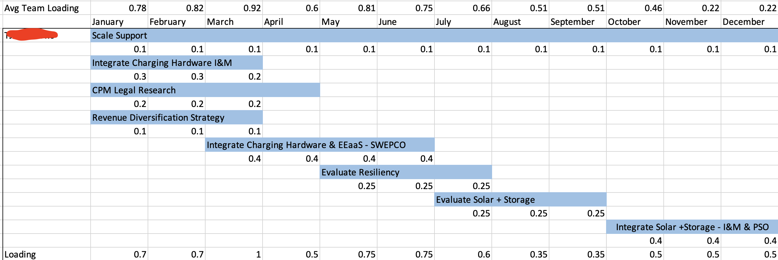
The screenshot above is done in EXCEL, and its calculating the allocation% percentage of each project by month for an individual. It also has a blue bar that highlights the months that have values in it.

I am trying to replicate this in smarthseet and I am not sure the best way to approach this or if its even possible to do in smarsheet. To be fair, in the excel screenshot above, there is no conditional format. Looks like someone manually highlighted the rows. Looking for a way to automate that in smartsheet whether calendar view, gnatt view, or even conditional format.

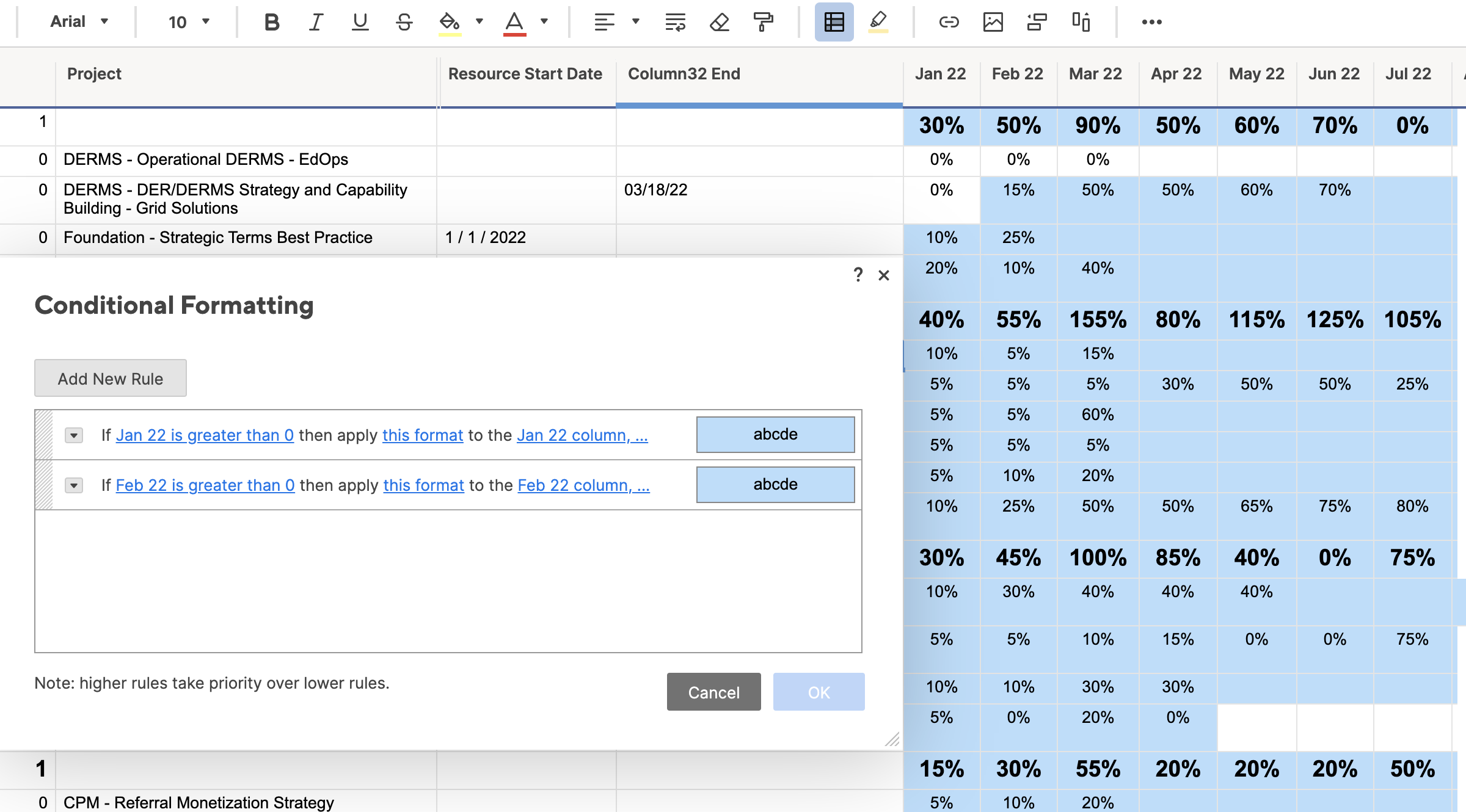
What I tried is in the screenshot below:

As seen in the second screenshot above, I have columns for every month and within those columns are values where the user can put their allocation percentage in for each project.

Is there a way to highlight the cells that have percentage values in like the excel example? I don't think calendar or gnatt view would work because those are based off of date columns and even though the columns I am using are months, they are not date columns.

Conditional formatting? Unfortunately there isn't an easy with to highlight multiple specific cells. Its either by row or one cell.

Paul Newcome

Yes. The conditional formatting has to be set up column by column.

As for the end date formula and needing to subtract 1 month from the end result, let's try this...

=IFERROR(DATE(YEAR([Resource Start Date]@row) + ROUNDDOWN((MONTH([Resource Start Date]@row) + COUNTIFS([Jan 22]@row:[Dec 23]@row, @cell > 0)) / 12, 0) + IF(IF(MOD(MONTH([Resource Start Date]@row) + COUNTIFS([Jan 22]@row:[Dec 23]@row, @cell > 0), 12) = 0, 12, MOD(MONTH([Resource Start Date]@row) + COUNTIFS([Jan 22]@row:[Dec 23]@row, @cell > 0), 12)) = 12, -1), IF(MOD(MONTH([Resource Start Date]@row) + COUNTIFS([Jan 22]@row:[Dec 23]@row, @cell > 0), 12) = 0, 12, MOD(MONTH([Resource Start Date]@row) + COUNTIFS([Jan 22]@row:[Dec 23]@row, @cell > 0), 12)) - 1, 28), DATE(YEAR([Resource Start Date]@row) + ROUNDDOWN((MONTH([Resource Start Date]@row) + COUNTIFS([Jan 22]@row:[Dec 23]@row, @cell > 0)) / 12, 0) + IF(IF(MOD(MONTH([Resource Start Date]@row) + COUNTIFS([Jan 22]@row:[Dec 23]@row, @cell > 0), 12) = 0, 12, MOD(MONTH([Resource Start Date]@row) + COUNTIFS([Jan 22]@row:[Dec 23]@row, @cell > 0), 12)) = 12, -1) + 1, 12, 28))

Paul Newcome

You can do a couple of different things...

You can insert 2 date type columns and use a formula to output a start and end date based on the first and last month filled in.

You can set up conditional formatting on a column by column basis to highlight the cells in each column that are not blank.

mbsamuel6

Hi Paul,

Thank you for the response. I apologize in advanced as I'm still very confused.

I would like to lean more to your first option. However, I'm not sure how I would do that.

So I create two date columns basically start and end date. Then in the start date column I would have a formula look at the range of cells from the Jan22 - Dec22. The formula would return the date of the first entry based off if there's a number greater then 0%?

Something like =if range of columns from Jan 22 - Dec 22 is greater then 0% return the date?

How would it return a date when those columns are not date columns and its not a date value?

I hope I'm not confusing you. Ha

Your second option sounds more easier, however the problem I'm running into with that is that it would highlight the entire column including the ones with the 0%. Where instead we would just want to highlight cells that are greater then 0%.

It be so much easier I think to say highlight any cells that has a value greater then 0% instead of an entire row or column.

Paul Newcome

The first one would be more of a nested IF statement within a DATE function.

=DATE(IF(OR([Jan 22]@row> 0, [Feb 22]@row> 0, [Mar 22]@row> 0, ................), 2022, IF(OR([Jan 23]@row> 0, [Feb 23]@row> 0, [Mar 23]@row> 0, ................), 2023)), IF(OR([Jan 22]@row> 0, [Jan 23]@row> 0), 1, IF(OR([Feb 22]@row> 0, [Feb 23]@row> 0), 2, ..............)))))))))))), 1)

The above is just an example of the basic structure assuming you have Jan 22 through Dec 23 on your sheet. It could be simplified if you only have one year or it can be expanded. Of course you would need to finish out the logic for each for each of the IF/OR statements, but it would follow the same pattern of the data that I included already.

The above is also only for the Start Date.

The below should give you the end date:

=DATE(YEAR([Start Date]@row) + ROUNDDOWN((MONTH([Start Date]@row) + COUNTIFS([Jan 22]@row:[Dec 23]@row, @cell> 0)) / 12, 0) + IF(IF(MOD(MONTH([Start Date]@row) + COUNTIFS([Jan 22]@row:[Dec 23]@row, @cell> 0), 12) = 0, 12, MOD(MONTH([Start Date]@row) + COUNTIFS([Jan 22]@row:[Dec 23]@row, @cell> 0), 12)) = 12, -1), IF(MOD(MONTH([Start Date]@row) + COUNTIFS([Jan 22]@row:[Dec 23]@row, @cell> 0), 12) = 0, 12, MOD(MONTH([Start Date]@row) + COUNTIFS([Jan 22]@row:[Dec 23]@row, @cell> 0), 12)), 28)

Paul Newcome

Looking at your conditional formatting rules, they seem to be set up correctly, but we need to figure out why it is highlighting the 0%. How exactly are each of the cells filled in?

mbsamuel6

Thanks again for the help. I'll test out that nested If statement in a few.

As for your question about the 0% all the cells are manually entered in. The only ones that were not manually entered are the ones in bold. The cells with the bold percentages in the month columns has a formula that Sums up the children rows.

mbsamuel6

And for that nested formula,

Getting an unparseable error.

=DATE(IF(OR([Jan 22]@row > 0, [Feb 22]@row > 0,[Mar 22]@row>0,[Apr 22]@row>0,[May 22]@row>0,[Jun 22]@row>0,[Jul 22]@row>0,[Aug 22]@row>0,[Sept 22]@row>0,[Oct 22]@row>0,[Nov 22]@row>0,[Dec 22]@row>0),2022,IF(OR([Jan 23]@row>0,[Feb 23]@row>0,[Mar 23]@row>0,[Apr 23]@row>0,[May 23]@row>0,[Jun 23]@row>0,[Jul 23]@row>0,[Aug 23]@row>0,[Sep 23]@row>0,[Oct 23]@row>0,[Nov 23]@row>0,[Dec 23]@row>0),2023)),IF(OR([Jan 22]@row>0,[Jan 23]@row>0),1,IF(OR([Feb 22]@row > 0,[Feb 23]@row>0),2,IF(OR([Mar 22]@row>0,[Mar 23]@row>0),3,IF(OR([Apr 22]@row>0,[Apr 23]@row>0),4,IF(OR(,[May 22]@row>0,[May 23]@row>0),5,IF(OR([Jun 22]@row>0,[Jun 22]@row>0),6,IF(OR(,[Jul 22]@row>0,[Jul 23]@row>0),7,IF(OR([Aug 22]@row>0,[Aug 23]@row>0),8,IF(OR([Sept 22]@row>0,[Sep 23]@row>0),9,IF(OR([Oct 22]@row>0,[Oct 23]@row>0),10,[Nov 22]@row>0,[Nov 23]@row>0),11,IF(OR([Dec 22]@row>0,[Dec 23]@row>0),12))))))))))),1)

And your assumption was correct. Only doing 2022 and 2023. Nice

mbsamuel6

Getting an unparsable error message for that start date formula.

=DATE(IF(OR([Jan 22]@row > 0, [Feb 22]@row > 0,[Mar 22]@row>0,[Apr 22]@row>0,[May 22]@row>0,[Jun 22]@row>0,[Jul 22]@row>0,[Aug 22]@row>0,[Sept 22]@row>0,[Oct 22]@row>0,[Nov 22]@row>0,[Dec 22]@row>0),2022,IF(OR([Jan 23]@row>0,[Feb 23]@row>0,[Mar 23]@row>0,[Apr 23]@row>0,[May 23]@row>0,[Jun 23]@row>0,[Jul 23]@row>0,[Aug 23]@row>0,[Sep 23]@row>0,[Oct 23]@row>0,[Nov 23]@row>0,[Dec 23]@row>0),2023)),IF(OR([Jan 22]@row>0,[Jan 23]@row>0),1,IF(OR([Feb 22]@row > 0,[Feb 23]@row>0),2,IF(OR([Mar 22]@row>0,[Mar 23]@row>0),3,IF(OR([Apr 22]@row>0,[Apr 23]@row>0),4,IF(OR(,[May 22]@row>0,[May 23]@row>0),5,IF(OR([Jun 22]@row>0,[Jun 22]@row>0),6,IF(OR(,[Jul 22]@row>0,[Jul 23]@row>0),7,IF(OR([Aug 22]@row>0,[Aug 23]@row>0),8,IF(OR([Sept 22]@row>0,[Sep 23]@row>0),9,IF(OR([Oct 22]@row>0,[Oct 23]@row>0),10,[Nov 22]@row>0,[Nov 23]@row>0),11,IF(OR([Dec 22]@row>0,[Dec 23]@row>0),12)))))))))),1)

mbsamuel6

Disregard the previous comment I got both the start date and end date to work.

Well the end date is working but it is off by one. Like its counting one month after the supposed end date:

=DATE(YEAR([Resource Start Date]@row) + ROUNDDOWN((MONTH([Resource Start Date]@row) + COUNTIFS([Jan 22]@row:[Dec 23]@row, @cell > 0)) / 12, 0) + IF(IF(MOD(MONTH([Resource Start Date]@row) + COUNTIFS([Jan 22]@row:[Dec 23]@row, @cell > 0), 12) = 0, 12, MOD(MONTH([Resource Start Date]@row) + COUNTIFS([Jan 22]@row:[Dec 23]@row, @cell > 0), 12)) = 12, -1), IF(MOD(MONTH([Resource Start Date]@row) + COUNTIFS([Jan 22]@row:[Dec 23]@row, @cell > 0), 12) = 0, 12, MOD(MONTH([Resource Start Date]@row) + COUNTIFS([Jan 22]@row:[Dec 23]@row, @cell > 0), 12)), 28)

mbsamuel6

And I know I shouldn't post multiple times in a row (I can't edit posts after a hour), but I did get the conditional format to work. I think its due to me having multiple columns selected when I picked which columns to color.

Basically to get it working right I had to go one by one for each month when making a new rule. Kind of a pain, but it worked.

Now the only issue I have is what I mentioned above. The resource end date being off by one.

But it seems to work fine in the Gnatt view once I create a report. So not a huge deal tbh

Paul Newcome

Yes. The conditional formatting has to be set up column by column.

As for the end date formula and needing to subtract 1 month from the end result, let's try this...

=IFERROR(DATE(YEAR([Resource Start Date]@row) + ROUNDDOWN((MONTH([Resource Start Date]@row) + COUNTIFS([Jan 22]@row:[Dec 23]@row, @cell > 0)) / 12, 0) + IF(IF(MOD(MONTH([Resource Start Date]@row) + COUNTIFS([Jan 22]@row:[Dec 23]@row, @cell > 0), 12) = 0, 12, MOD(MONTH([Resource Start Date]@row) + COUNTIFS([Jan 22]@row:[Dec 23]@row, @cell > 0), 12)) = 12, -1), IF(MOD(MONTH([Resource Start Date]@row) + COUNTIFS([Jan 22]@row:[Dec 23]@row, @cell > 0), 12) = 0, 12, MOD(MONTH([Resource Start Date]@row) + COUNTIFS([Jan 22]@row:[Dec 23]@row, @cell > 0), 12)) - 1, 28), DATE(YEAR([Resource Start Date]@row) + ROUNDDOWN((MONTH([Resource Start Date]@row) + COUNTIFS([Jan 22]@row:[Dec 23]@row, @cell > 0)) / 12, 0) + IF(IF(MOD(MONTH([Resource Start Date]@row) + COUNTIFS([Jan 22]@row:[Dec 23]@row, @cell > 0), 12) = 0, 12, MOD(MONTH([Resource Start Date]@row) + COUNTIFS([Jan 22]@row:[Dec 23]@row, @cell > 0), 12)) = 12, -1) + 1, 12, 28))

mbsamuel6

That worked!!!! Words cannot describe how thankful I am for this. Those formulas will help so much going forward.

Paul Newcome

Happy to help. 👍️