My first automatic RYG/RAG schedule status formulas

CanadaJim

Hi everyone.

This is my first new discussion. I wanted to share some automation I put into my schedule that made it much more friendly.

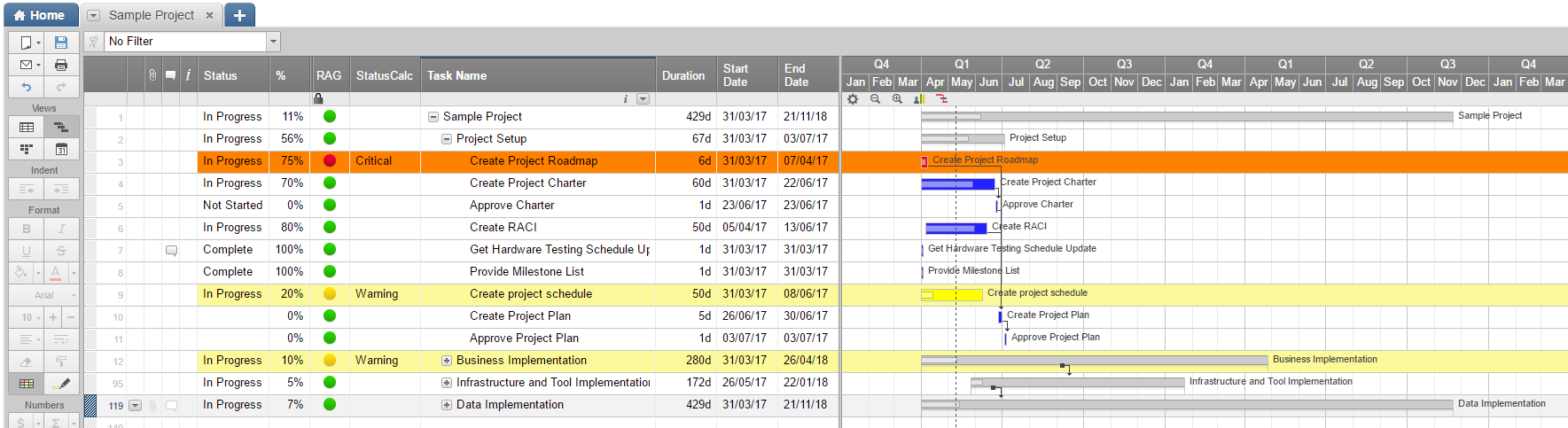
First, I have a few key columns:

1. Status (Drop-down, manual entry, "Not Started" or "In Progress" or "Completed")
2. % (Manual, progress on completing a task)
3. RAG (Automatic, shows Red, Amber or Green based on a formula)
4. StatusCalc (Text field, Automatic, Key formula to determine whether a task is Warning or Critical)
5. Start/End Dates (Standard fields, used in calculations)

StatusCalc Formula:

=IF(OR(Status1 = "Complete", [End Date]1 = [Start Date]1), "", IF(AND([End Date]1 < (TODAY(0) + 1), %1 < 1), "Critical", IF(OR(AND(OR(Status1 = "", Status1 = "Not Started"), [Start Date]1 < TODAY(0)), (TODAY(0) - [Start Date]1) / ([End Date]1 - [Start Date]1) > %1), "Warning", "")))

To break it down, it goes like this:

1. If the status has manually been set to "Complete" or it's a milestone (0 day activity), I assume it is not in Warning or in Critical.  For some, milestones may still be warning or critical, but without baseline versus actual calculations I'd rather focus on the tasks.
2. If the end date is tomorrow or sooner, and % is less than 100%, I flag the task Critical.
3. The next one is the trickiest.  It has 2 conditions for Warning:
   1. Status is blank or "Not Started", and start date was earlier than today, it's Warning.
   2. The next formula calculates the percentage of time elapsed versus the percentage complete.  If percent elapsed is more than percent complete (I.e. more time has run out than work completed), it goes into Warning.  This is helpful for focusing on the challenged tasks.

Next, I have a simple formula in the RAG/RYG column:

=IF(StatusCalc1 = "Warning", "Yellow", IF(StatusCalc1 = "Critical", "Red", "Green"))

It's pretty basic, and sets the colour of the flag to Red, Yellow/Amber or Green based on the previous status calculation.

Finally, I set a column and gantt conditional formatting based on the RAG to highlight warning tasks a lighter yellow and critical tasks a lighter red.  This makes it very easy to quickly review the schedule and identify problem tasks to focus on.

I hope this helps some of you get some additional functionality out of this tool.

Jim

Ben W

Thanks Jim, really appreciate you sharing.

JennAnderson

Hi Jim,  

I love this concept!  When I try to copy in the StatusCalc formula, it doesn't seem to be recognizing my column values (i.e. the text in the formula doesn't highlight the data boxes like it would for an active formula).  Any ideas?

CanadaJim

Hi Jenn.

If you just copy and paste the formula, it may not work because you have different column names.

Can you please tell me the names of the columns in your table you want to use?

Do you get an error message in the cell, or does it just show the formula in the cell?

By the way, I also consolidated this solution a bit to not require the "StatusCalc" column.  Once you let me know the answers to the above, I'll share the update with you.

CanadaJim

Here's the update I mentioned above.

I realized a short time after posting this that the StatusCalc formula can be contained entirely in the RAG column, just changing the values in the formula to the colour name (Green, Yellow, Red) instead of the status (On Track, Warning, Critical).

Then you can remove the StatusCalc column entirely.

So the RAG/RYG formula looks like this:

=IF(OR(Status1 = "Complete"; [End Date]1 = [Start Date]1); "Green"; IF(AND([End Date]1 < (TODAY(0) + 1); %1 < 1); "Red"; IF(OR(AND(OR(Status1 = ""; Status1 = "Not Started"); [Start Date]1 < TODAY(0)); (TODAY(0) - [Start Date]1) / ([End Date]1 - [Start Date]1) > %1); "Yellow"; "Green")))

JenValdez

This was extremely helpful. How would I adapt the formula to also include the status of "In Progress", in which the RYG/StatusCalc status would be determined by how far away from the Finish/End Date we are. 

Currently I have a task with the status as In Progress, at 75%, it's showing as Critical (we're way past the due date) but showing Green circle. 

Looking forward to your recommendations!

RawRobb

Hi Jim, love this, exactly what i'm looking for however i'm getting #unparseable when i try to copy this into the cell.  I have same headings as you minus the duration column.  

Thank you