Sign in to join the conversation:
Hi there Smartsheet Guru's!
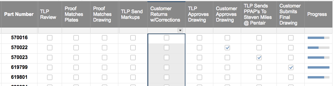
Im trying to figure out the best way to automate a progress bar, based of 9 columns that all have check boxes. Screenshot shown:
Here's an idea I just tried out that might work for you: You can automate the progress bar using a formula in conjunction with the progress status symbol column type. You can add a column that calculates the percentage completion of the nine tasks, called "% Complete". The formula for the first row would be:
=COUNTIF([TLP Review]1:[Customer Submits Final Drawing]1,1)/9
Then, you can reference this "% Complete" column in your progress column, which should be a symbol column with the progress bar status type selected. You can use the following formula:
=IF([% Complete]1 < 0.25, "Empty", IF([% Complete]1 < 0.5, "Quarter", IF([% Complete]1 < 0.75, "Half", IF([% Complete]1 < 1, "Three Quarter", "Full"))))
This will select the appropriate progress bar level for the percent complete - "Empty" if the % complete is between 0 and .25, "Quarter" for .25 to .5, etc. You can then hide the "% Complete" column if needed.
I would suggest using a COUNTIFS statement within a nested IF statement. Something along the lines of
=IF(COUNTIFS([TLP Review]@row:[Customer Submits Final Drawing]@row, 1) < 1, "Empty", IF(COUNTIFS([TLP Review]@row:[Customer Submits Final Drawing]@row, 1) < 3, "Quarter", IF(COUNTIFS([TLP Review]@row:[Customer Submits Final Drawing]@row, 1) < 6, "Half", IF(COUNTIFS([TLP Review]@row:[Customer Submits Final Drawing]@row, 1) < 9, "Three Quarter", "Full"))))
This will give you the following results depending on how many boxes are checked (feel free to adjust the numbers as desired):
0 = Empty
1 = Quarter
2 = Quarter
3 = Half
4 = Half
5 = Half
6 = Three Quarters
7 = Three Quarters
8 = Three Quarters
9 = Full
This is it! I would still be fumbling with the formula. I was using countif not countifs and, I wasnt using @row. It works perfectly. Thank you!
Happy to help. I personally never use COUNTIF anymore. COUNTIFS works even with the one set of criteria, and I can just plug any extras in as needed without having to worry about forgetting to put the "S" on there.
@row is super useful in MOST cases. The only time I specify a row number anymore is when I need to reference a different row. It makes a lot of things so much easier to include testing and whatnot.
Hey Paul - Trying to apply your logic to this issue. Can you tell where I fumbled?
I'm trying to create a % formula that will calculate the % complete of task / row based on the number of checkboxes that have been checked.
For example- I used 7 checkboxes for 7 task rows:
5 = Three Quarters
7 = Full
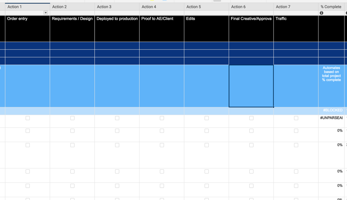
**I tried below harvey ball formula and rec'd an "unparseable" error....
=IF(COUNTIFS([Action 1]@row:[Action 7]@row, 1) < 1, "Empty”, IF(COUNTIFS([Action 1]@row:[Action 7]@row, 1) < 3, "Quarter”, IF(COUNTIFS([Action 1]@row:[Action 7]@row, 1) < 6, "Half”, IF(COUNTIFS([Action 1]@row:[Action 7]@row, 1) < 9, "Three Quarter", "Full"))))
Thank you in advance.
~Amy
You say "7 task rows". Is it actually 7 rows or is it 7 columns going across the row?
Other than that, your syntax is correct and your column names/ranges are consistent. Without a screenshot, that would be my first question.
Should your ranges be
7 checkbox columns across the same row?
[First Check Column]@row:[Last Check Column]@row
.
or should it be 7 checkboxes down the same column?
[Check Column]1:[Check Column]7
Here is a screenshot....might clarify. Thanks for your help. I'm running around in circles.
That's really odd. Everything appears to be absolutely correct.
Lets try this... Take the next four cells below it, and enter each individual IF statement into it's own row. If only one throws an error then it narrows down where the issue could be. If they all throw an error, we may need to break it down even further or start thinking a little outside of the box.
Ok- the first 3 statements did not work, but the last one DID -
=IF(COUNTIFS([Action 1]@row:[Action 7]@row, 1) < 9, "Three Quarter", "Full")
Recommendations on putting them together? I must be missing something simple.
TY again!
So this is what you have...
=IF(COUNTIFS([Action 1]@row:[Action 7]@row, 1) < 1, "Empty”)
=IF(COUNTIFS([Action 1]@row:[Action 7]@row, 1) < 3, "Quarter”)
=IF(COUNTIFS([Action 1]@row:[Action 7]@row, 1) < 6, "Half”)
and only the last one is working?
Temporarily change the column type to text/number and just do the COUNTIFS in a row.
=COUNTIFS([Action 1]@row:[Action 7]@row, 1)
Check random boxes within that row to make sure the COUNTIFS is working.
You can even drag this down the rows and have each row a different number of boxes checked.
If the COUNTIFS is what is failing, try changing the criteria to true.
=COUNTIFS([Action 1]@row:[Action 7]@row, true)
Thanks Paul - I appreciate your time and thinking!
Sure thing! Did this solve the issue?
@Paul Newcome - I want to do something really similar. I want to COUNTIF the cells in each column are green 'Checked Ok' and adjust the progress bar based on the number of these. Any help would be very gratefully received! ty
@Miranda Rais You are going to first use a COUNTIFS to count how many meet your criteria then use that as a part of the "logical statement" portions within a nested IF statement.
=IF(COUNTIFS([We View]@row:[Sports App IOS]@row, "Checked Ok") = 0, "output_if_zero", IF(COUNTIFS([We View]@row:[Sports App IOS]@row, "Checked Ok") = 1, "output_if_one", IF(COUNTIFS([We View]@row:[Sports App IOS]@row, "Checked Ok") = 2, "output_if_two", ...............................
You are going to need to change the "output_if_#" portions to output whatever you want for each number and continue the pattern until you have an output for each of the different possible counts.
*IDs have been omited for privacy but there are values in the column I need to bring in the Week # values from the Master Tracker - 2026 sheet into the Week-Over-Week Modified sheet. The group and APC ID need to match. There is a potential of duplicate APC values which is why I need the group to be a criteria as well. I…
I have one sheet that is tracking PTO where a user has entered the days off. The form allows them to enter a start and end date for their PTO and enters a single record into the sheet. I have a second sheet that I am looking to pull that data into, but there is only one record per person (column in this sheet where the…
I am trying to get the passenger count per month per year, and I can't seem to get the formula correct. I need to add the number of passengers for each month per year. If anyone could assist me with this, I would greatly appreciate it. Thanks!