Auto fill cells based on multiple criteria, using Index Match

I'm struggling with the logic here so any help is appreciated.

My team manages new hires and we have to rate their performance weekly to report back to the new hires respective manager. Our program is 10 weeks long and to consistently rate them on the same metrics week to week, we created a survey that the trainers would fill out once per week per trainee. It ends up in a grid like this:

In this same form, I've created helper columns to convert the star ratings to a numeric value:

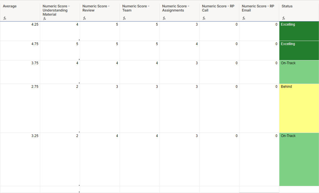
Pretty straight forward.


Now, the complex part is all the New Hires go into one form. We have up to 4 new hire classes going on at once and trainers inputting data at the same time. I want to extract the metrics per trainee into a separate sheet per class.

Here's what I've got so far:

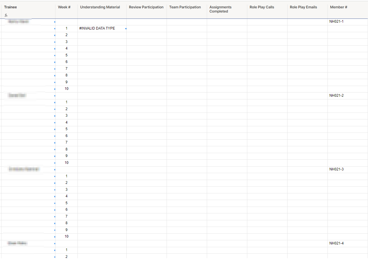
So the Trainee column is populated with a formula using Index Match to pull from our Master NH tracking sheet using the Member Number.

Then, I created a row for each week for each New Hire. In the next 6 columns, I want to pull from the specific Numeric Column for the user per week that was input by the trainer.

For example, the Trainer puts in that NH021-1 received a 4 for Understanding Material in Week 1, then a 4 would appear in Column3, Row2 (where the error message is currently)


Here's the formula I currently have:

=INDEX({Status - UM}, AND(MATCH(Trainee1, {Status - Name}, 0), MATCH([Week #]@row, {Status - Week}, 0)))

I tried using AND to Match twice, once for the Name of the Trainee, and again for the week.


I'm familiar with SQL querying so I'm struggling not being able to use WHERE clauses.

Thanks in advance for the help!

Best Answers

  • Paul Newcome
    Paul Newcome ✭✭✭✭✭✭
    Answer ✓

    You are going to need an INDEX/COLLECT.


    =INDEX(COLLECT({Range to pull from}, [1st criteria range}, 1st criteria, {2nd criteria range}, 2nd criteria), 1)

  • dhall
    dhall ✭✭✭
    Answer ✓

    Oh neat. Didn't think about Index/Collect.

    I did get it to work with INDEX/MATCH. On my form sheet, I created a new column with a column formula that took the "Name" and "Week" ( =[Name]@row+[Week]@row) and added them together, so it creates a unique code. For example, "Bob Bobberson" for name and "3" for week, becomes "Bob Boberson3", which I've deemed as the {Status - Unique} column through the sheet references.

    Then, in the destination sheet, I put in the MATCH formula to look for "[TraineeName]@<rownumber> + <week>, {Status - Unique}, 0"

    So it looks like this now:

    =IFERROR(INDEX({Status - UM}, MATCH([Trainee / Metric]1 + 2, {Status - Unique}, 0)), "-")

    {Status - UM} pulls the column I care about for the Metric, followed by the MATCH to get the exact row.

    The IFERROR is there because I don't want my sheet populated with #NOMATCH while we wait for the next input of data.


    I'll have to try out the INDEX/COLLECT on something though! Thanks for the input!

Answers

  • dhall
    dhall ✭✭✭

    I should specify the end goal as well.

    To easily create reports for managers per class/per trainee, we need to get the data out of the form.

    From what I can tell with dashboards, there is no easy way to create a metric or chart showing progression, which is why I created the second sheet for the class with all the Weeks in individual rows as above.

    I'll take suggestions on how to format this as well, to make it cleaner and easier to manage and manipulate as we have more classes in the future.

  • Paul Newcome
    Paul Newcome ✭✭✭✭✭✭
    Answer ✓

    You are going to need an INDEX/COLLECT.


    =INDEX(COLLECT({Range to pull from}, [1st criteria range}, 1st criteria, {2nd criteria range}, 2nd criteria), 1)

  • dhall
    dhall ✭✭✭
    Answer ✓

    Oh neat. Didn't think about Index/Collect.

    I did get it to work with INDEX/MATCH. On my form sheet, I created a new column with a column formula that took the "Name" and "Week" ( =[Name]@row+[Week]@row) and added them together, so it creates a unique code. For example, "Bob Bobberson" for name and "3" for week, becomes "Bob Boberson3", which I've deemed as the {Status - Unique} column through the sheet references.

    Then, in the destination sheet, I put in the MATCH formula to look for "[TraineeName]@<rownumber> + <week>, {Status - Unique}, 0"

    So it looks like this now:

    =IFERROR(INDEX({Status - UM}, MATCH([Trainee / Metric]1 + 2, {Status - Unique}, 0)), "-")

    {Status - UM} pulls the column I care about for the Metric, followed by the MATCH to get the exact row.

    The IFERROR is there because I don't want my sheet populated with #NOMATCH while we wait for the next input of data.


    I'll have to try out the INDEX/COLLECT on something though! Thanks for the input!

Help Article Resources

Want to practice working with formulas directly in Smartsheet?

Check out the Formula Handbook template!