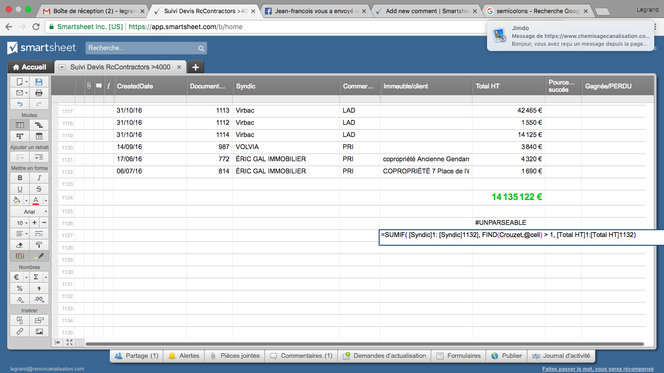
##Help ME please "i can t continue to work" SumIF##

ArnaudLegrand

I post a problem 2 days ago 

some response but still doesn t work, new to smartsheet but my work is blocke now

 

problem

Hello @Craig and other Helpers

i experiment the same issue than other

sorry for my english but i m french

i copy your formula below and try to adapt with "laserjet" type

i want to make a sum if a name appear in the row i write it but doesn t work

=SUMIF( [Syndic]1: [Syndic]1132]; FIND("Crouzet"; @cell) > 1; [Total HT]1:[Total HT]1132)

in order to find "Crouzet" wich is a part of name ex "Crouzet Breil"

I m new to Smartsheet et don t understand why

Appriciate help of community

after i will reuse the same formula to make some with different type of  name exemple "foncia", "taboni" but can appeat in row "cabinet Foncia" , or "cabinet Taboni"

regards

return error is #unparseable

legrand@renovcanalisation.com

 

Solution from Mike Wilday ,he s very kind but doesnt work

 

0

 

Try removing the brackets off of Syndic like this... brackets should only be used if the column name contains a space. 

=SUMIF(Syndic1:Syndic1132], FIND("Crouzet",@cell) > 1, [Total HT]1:[Total HT]1132)

There was also a space character after the first colon. Both of those could have been the issue. Also, the Find function should have "quotes" around the text you are searching for. Let me know if it works now. 

 

RESPONSE

0

 

hello Mike thank you so much

but .. doesnt work 

i think you understand my goal to make sum by name

THANK YOU VERY MUCH

HELP HELP HELP

M

 

 

Mike Wilday

Hi Amaud, I hadn't responded because I had hoped another individual would chime in. I can't seem to get the formula with Find work. As a workaround,

1. You can create a new column çalled Crouzet and place the find formula =Find("Crouzet", Syndic1) in the first field of that column.

2. Use the little square in the bottom-right (or double-click it) to fill the formula all the way down)

2. Hide the column if you don't want to see it in your view.

3. Then use this formula to sum your =Sumif(crouzet1:crouzet1132, 1, [Total HT]1:[Total HT]1132)

I was able to get this done in my example. 

ArnaudLegrand

thank you for your help but maybe my word are no clear , it s not why i try to do or i don t understand ..

i ask the support to help

thank you so much

 

Mike Wilday

Hi Amaud, because I couldn't get the Find formula to work in sumif, I used the find formula in its own column the second column containing the 1's. That column is checking if the first column contains Crouzet. If it does, it gets a 1.

Then in your summary section, on your chart you can use this formula to check for the one's and then sum their Total HT if they are there. 

=Sumif(crouzet1:crouzet1132, 1, [Total HT]1:[Total HT]1132)

Mehmet Zengin

I just wanted to share something interesting I found while trying to make FIND work for this problem.

I tried to use newly published COLLECT function to see if it may work with FIND.

As seen on the screenshot when I search for "Cabinet", formula works perfectly.

=SUM(COLLECT([Total HT]1:[Total HT]4, Syndic1:Syndic4, FIND("Cabinet", @cell) = 1))

However, if I try with "CROUZET" it doesn't because I assume "CROUZET" isn't a recognized word and Smartsheet underline it with red even while you type it into the formula.

Update: Looks like I am partially wrong. It doesn't work for "RESIDENCE" but it works for "AIA". I would like to have support's comment on this.