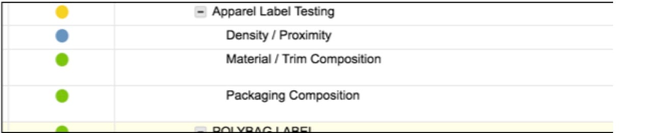
Formulas - Can you exclude rows from average calculations?

I am looking for the parent row to reflect a rollup of child row status color (RYG) AND if ALL child rows are blue (complete), have the parent row blue. I'm almost there, however, in the screenshot example below, the parent task is yellow although the 3 child tasks are either green (on track) or blue (complete).

Since the formula weights the different colors (R=0, Y=1, G=2) and divides the sum by the total number of child rows, the blue (completed) rows are counting against us in our average calculations.

Is there a way to re-write the formula to exclude blue rows from the average calculation?

=IFERROR(IF((COUNTIF(CHILDREN(), "Blue")) = COUNT(CHILDREN()), "Blue", IF((COUNTIF(CHILDREN(), "Yellow") + (COUNTIF(CHILDREN(), "Green") * 2)) / COUNT(CHILDREN()) <= 0.5, "Red", IF((COUNTIF(CHILDREN(), "Yellow") + (COUNTIF(CHILDREN(), "Green") * 2)) / COUNT(CHILDREN()) <= 1.5, "Yellow", IF((COUNTIF(CHILDREN(), "Yellow") + (COUNTIF(CHILDREN(), "Green") * 2)) / COUNT(CHILDREN()) <= 2.5, "Green")))), "-")

Example 1.jpg

Find more posts tagged with

Formulas

Comments

Paul Newcome

Yes. You just need to get the count of the blue children and subtract from the count of the children when setting your count for the IF statements.

..........(COUNTIF(CHILDREN(), "Green") * 2)) / (COUNT(CHILDREN()) - COUNTIF(CHILDREN(), "Blue")) <= 0.5, "Red".................

mailene.h

So helpful - thank you! I am now noticing that if the status color for the child rows are BLANK, then the parent will still turn blue (I would rather have it "-" or something). Do you have a recommendation to fix that?

Here is the latest formula:

=IFERROR(IF((COUNTIF(CHILDREN(), "Blue")) = COUNT(CHILDREN()), "Blue", IF((COUNTIF(CHILDREN(), "Yellow") + (COUNTIF(CHILDREN(), "Green") * 2)) / (COUNT(CHILDREN()) - COUNTIF(CHILDREN(), "Blue")) <= 0.5, "Red", IF((COUNTIF(CHILDREN(), "Yellow") + (COUNTIF(CHILDREN(), "Green") * 2)) / (COUNT(CHILDREN()) - COUNTIF(CHILDREN(), "Blue")) <= 1.5, "Yellow", IF((COUNTIF(CHILDREN(), "Yellow") + (COUNTIF(CHILDREN(), "Green") * 2)) / (COUNT(CHILDREN()) - COUNTIF(CHILDREN(), "Blue")) <= 2.5, "Green")))), "-")

Example 2.png

Paul Newcome

If all children are blank, then the count will be 0. So if you incorporate in there somewhere...

IF(COUNT(CHILDREN()) = 0, "-", ..........

Another option would be to add the criteria to the third portion of your last IF statement.

............IF((COUNTIF(CHILDREN(), "Yellow") + (COUNTIF(CHILDREN(), "Green") * 2)) / (COUNT(CHILDREN()) - COUNTIF(CHILDREN(), "Blue")) <= 2.5, "Green", "-")))), "-")

EEGordon

So what if your children are numbers that you want to average but you want to exclude rows where there is no value from the row count so it doesn't skew the average, but you need the row there chronologically?

This is the formula I was trying to use but it's not working

=(SUM(CHILDREN() / (COUNTIF(CHILDREN(), >=0))))

SS average exclusion.PNG

Paul Newcome

You could use something along the lines of

COUNTIFS(CHILDREN(), ISNUMBER(@cell))

This will only count children rows that have a number, so it will exclude text and blanks.

Sign in to join the conversation!

Quick Links

Trending discussions

Getting error message in approval email
Hey, Is anyone else facing this issue in the approval notifications sent through smartsheet
Add Package Count Based on Customer
I have a sheet with a list of customers in one column, and then the following columns are City, Monday, Tuesday, Wednesday, Thursday, Friday. I need help with a formula that I can put in my sheet summary so that if the customer column says Staples (It can say this in multiple rows) that it will tell me the total package…
Issue with automation process reporting a date in a special column
In the Smartsheet sheet “CRS RO Master” we have programmed an automation called “Track Changes in dates, confirmation and LHG code” [PICTURE 1] This one should report a date of a change in the columns “CRS GO LIVE DATE” and “PMS Go LIVE DATE” in the column “. CRS Check date changed”. [PICTURE 2] The update of the “Go live…