Current Task Formula based off certain criteria (symbols)

Hi,

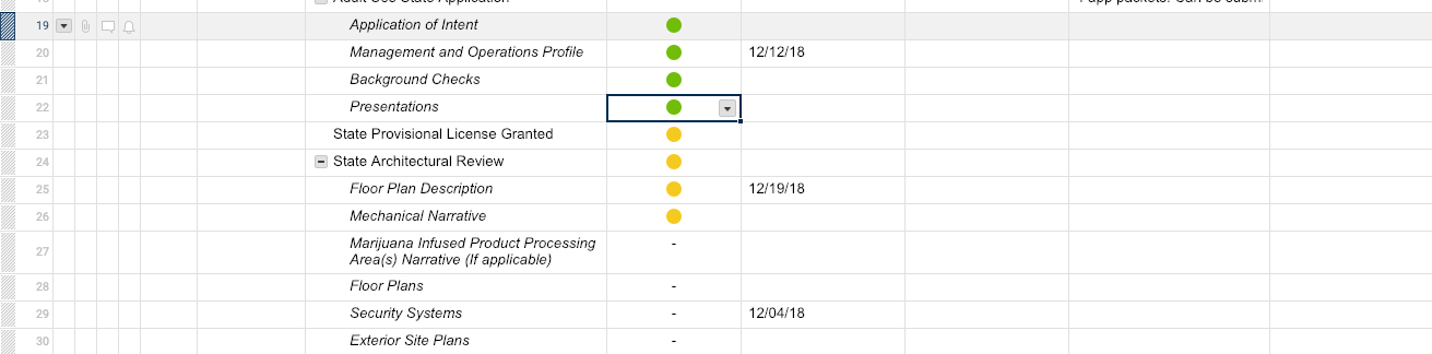
I want to create a formula that would read all rows have a Green symbol and read back the last task name that has green. This would have to be based off the row number and not dates, given not every task will have a start or end date.

Attachment for context --> I would want the formula to read all of those tasks and deliver back "presentations task" since that is the last Green row.

Screen Shot 2018-12-17 at 6.28.49 PM.png

Find more posts tagged with

Formulas

Reports

Project Management

Comments

Paul Newcome

Would it be possible to have a few greens, a few yellows, then a few more greens? If so, how would you determine which is the last green? If not I would assume that row 2 will never be green before row 1, row 3 would never be green before row 2, etc.

Both scenarios are possible to account for in a formula, but they do require very different formulas.

Frank_Mattiace

Hi Paul,

Thanks for helping out. I'd say having green come after a yellow status would be unlikely. The goal is to show the last green row. This would be based on the number of the row. So green in row 22 would be the last and the row I'd like to show. This formula would have to update as tasks are checked off as green.

Paul Newcome

Ok. And are all of the rows you are looking at children rows of another, or are you strictly looking at them as individual rows with the intention of having the last one marked green displayed elsewhere on the sheet such as at the top or in a summary?

Brian W

I’m curious what Paul comes up with but here is what I would do:

I would create a helper column that checks if the current row’s cell in the RYG column is green and counts the greens in the cells below that one. If the cell is green and there are 0 green cells below it, it assigns a 1. This formula goes in the first cell of the helper column and assumes you have 50 rows of data:

=IF(AND(RYGColumn1 = "green", COUNTIF(RYGColumn2:RYGColumn$50, ="green") < 1), 1,0)

Then I would use INDEX/MATCH to find the 1 in the GreenHelper column and return the corresponding cell in the Number column:

=INDEX(Number:Number, MATCH(1, GreenHelper:GreenHelper))

Paul Newcome

@Brian

If they are all children rows that are being looked at, and the data will be displayed in the parent row along side the parent row task, and there will never be a green lower than a yellow, then I would be joining the parent row task text with the child row task with something along the lines of

="Parent Row Text - " + INDEX(CHILDREN(), COUNTIFS(CHILDREN([RYG Column Name]@row), "Green"))

Using the screenshot provided in the original post, the Parent cell would read something along the lines of

Parent row text from row 18 - Presentations

Sign in to join the conversation!

Quick Links

Trending discussions

Dynamic formula to return date of next Thursday every week.
I'm wondering if anyone has worked out a dynamic formula to return the date of the 'next' Thursday of the month. I have a worksheet where I need to send out a reminder to a contacts in a contact column in the worksheet each Thursday of the current month if a criteria has not been met. When criteria has been met, then…
Check box for date in previous month
Hello, I have the formula to check a box for line items with the current month. =IF(AND(YEAR(Date@row ) = YEAR(TODAY()), MONTH(Date@row ) = MONTH(TODAY())), 1, 0) Trying to set up a report for all items with the previous month (i.e. 1 month prior to current). How can I modify to check the box?
Need Help with If, Index, Collect
Please help, I have a few of these to do. I have a nested IF formula. The first part is an INDEX/MATCH and works as a standalone. The next few are INDEX/COLLECT. These are not working as standalone or in the nested version (Unparsable Error). Any ideas? =IF(CONTAINS(“A/V”, [Vendor Type]@row ), INDEX(COLLECT({Date Secured…